arXiv:1511.06545v1 [cs.CV] 20 Nov 2015
A dense subgraph based algorithm for compact salient image region detection Souradeep Chakraborty* Department of Electronics and Electrical Communication Engineering, Indian Institute of Technology, Kharagpur 721302, India Email :
[email protected]
Pabitra Mitra Department of Computer Science and Engineering, Indian Institute of Technology, Kharagpur 721302, India Email :
[email protected]
Abstract We present an algorithm for graph based saliency computation that utilizes the underlying dense subgraphs in finding visually salient regions in an image. To compute the salient regions, the model first obtains a saliency map using random walks on a Markov chain. Next, k-dense subgraphs are detected to further enhance the salient regions in the image. Dense subgraphs convey more information about local graph structure than simple centrality measures. To generate the Markov chain, intensity and color features of an image in addition to region compactness is used. For evaluating the proposed model, we do extensive experiments on benchmark image data sets. The proposed method performs comparable to well-known algorithms in salient region detection. Keywords: Visual saliency, Markov chain, Equilibrium distribution, Random walk, k-dense subgraph, Compactness
1. Introduction The saliency value of a pixel in an image is an indicator of its distinctiveness from its neighbors and thus its ability to attract attention. Visual attention has been successfully applied to many computer vision applications, e.g. adaptive image compression based on region-of-interest [35], object recognition [36,37,38], and scene classification [39]. Nevertheless, salient region and object detection still remains a challenging task. The goal of this work is to extract the salient regions in an image by combining superpixel segmentation and a graph theoretic saliency computation. Dense subgraph structures are exploited to obtain an enhanced saliency map. First, we segment the image into regions or superpixels using the SLIC (Simple Linear Iterative Clustering) superpixel segmentation method [19]. Then we obtain a
Preprint submitted to Elsevier
November 23, 2015
saliency map using the graph based Markov chain random walk model proposed earlier [1], considering intensity, color and compactness as features. Using this saliency map, we create another sparser graph, on which k-dense subgraph is computed. We get a refined saliency map by this technique. The use of dense subgraph on a graph constructed from segmented image regions helps to filter out the densely salient image regions from saliency maps. A number of graph based saliency algorithms are known in literature that improvise on the dissimilarity measure to model the inter-nodal transition probability [1], provide better random walk procedures like random walk with restart [18], or use combinations of different functions of transition probabilities e.g., site rate entropy function [14] to build their saliency model. However, most graph based methods produce a blurred saliency map. It would be useful to postprocess the map to filter out the most salient portions. Our model also being a graph based method, uses dense subgraph computation to filter out salient regions after random walk is employed. The suppression of non-salient regions combined with salient region shape retention, yields saliency maps more closely resembling ground truth data as compared to the existing methods used for comparison. This has been achieved by considering a more informative local graph structure, namely, dense subgraphs, than simple centrality measures in obtaining the map. The remainder of the paper is organized as follows. Section 2 surveys some previously proposed saliency detection algorithms. Section 3 describes the proposed saliency detection procedures. Section 4 is devoted to experimental results and evaluation. We demonstrate that the proposed method achieves superior performance when compared to well-known models, on standard image data sets and also preserves the overall shapes and details of salient regions quite reliably. Finally in section 5, we conclude this paper with future research issues. 2. Related Work Saliency computation is rooted in psychological theories about human attention, such as the feature integration theory (FIT) [44]. The theory states that, several features are processed in parallel in different areas of the human brain, and the feature locations are collected in one “master map of locations”. From this map, “attention” selects the current region of interest. This map is similar to what is nowadays called “saliency map”, and there is strong evidence that such a map exists in the brain. Inspired by the biologically plausible architecture proposed by Koch and Ullman [45], mainly designed to simulate eye movements, Itti et al. [3] introduced a conceptually computational model for visual attention detection. It was based on multiple biological feature maps generated by mimicking human visual cortex neurons. It is related to the FIT theory [44] which outlines the human visual search strategies. The recent survey by Borji and Itti [47] lists a series of visual attention models [47], which demonstrate that eye-movements are guided by both bottom-up (stimulus-driven) and top-down (task-driven) factors.
2
Region based saliency models have been proposed in a number of works. The early work of Itti et al. [3] was extended by Walther and Koch [15] who proposed a way to extract proto-objects. Proto-objects are defined as spatial extension of the peaks of this saliency map. This approach calculates the most salient points according to the spatial-based model, henceforth the saliency is spread to the regions around them. The work in [31] addresses the problem of detecting irregularities in visual data, e.g., detecting suspicious behaviors in video sequences, or identifying salient patterns in images. The problem is posed as an inference process in a probabilistic graphical model. The framework in [1], is a computer vision implementation of the object based attention model of [6]. In this paper, a grouping is done by conducting a segmentation method, which acts as the operation unit for saliency computation. In [7], the problem of feature map generation for region-based attention is discussed, but a complete saliency model has not been proposed. The method in [8] is based on preattentive segmentation, dividing the image into segments, which serve as candidates for attention, and a stochastic model is used to estimate saliency. In [9], visual saliency is estimated based on the principle of global contrast, where the region is employed in computation and is used primarily for the sake of speed up. In the work [23], two characteristics: rareness and compactness have been utilized. In this approach, rare and unique parts of an image are identified, followed by aggregating the surrounding regions of the spots to find the salient regions thus imparting compactness to objects. In the method followed in [22], saliency is detected by over-segmenting an image and analyzing the color compactness in the image. Li et al., in their work [33], offer two contributions. First, they compose an eye movement dataset using annotated images from the PASCAL dataset [54]. Second, they propose a model that decouples the salient object detection problem into two processes: 1) a segment generation process, followed by 2) a saliency scoring mechanism using fixation prediction. A novel propagation mechanism, dependent on Cellular Automata, is presented in [34] which exploits the intrinsic relevance of similar regions through interactions with neighbors. Here, multiple saliency maps are integrated in a Bayesian framework. Several graph based saliency models have been suggested so far. It is shown in [10] that gaze shift can be considered as a random walk over a saliency field. In [11], random walks on graphs enable the identification of salient regions by determining the frequency of visits to each node at equilibrium. Harel et al. [1] proposed an improved dissimilarity measure to model the transition probability between two nodes. These kinds of methods consider information to be the driving force behind attentive sampling and use feature rarity to measure visual saliency. In this article, we base our model on such a graph based model and utilize the embedded dense subgraphs to better extract the most salient regions from an image. The work in [12] provides a better scheme to define the transition probabilities among the graph nodes and thus constructs a practical framework for saliency computation. Wang et al. [14] generated several feature maps by filtering an input image with sparse coding basis functions. Then they computed the overall saliency map by multiplying saliency maps obtained us3
ing two methods: one is the random walk method and the other based on the entropy rate of the Markov chain. Gopalakrishnan et al. [12], [13] formulated the salient region detection as random walks on a fully connected graph and a k-regular graph to consider both global and local image properties in saliency detection. They select the most important node and background nodes and used them to extract a salient object. Jiang et al. [30] consider the absorption time of the absorbing nodes in a Markov chain (constructed on a region similarity graph) and separate the salient objects from the background by a global similarity measure. Yang et al. [29] ranks the similarity of the image regions with foreground cues or background cues via graph-based manifold ranking, and detects background region and foreground salient objects. In a more recent work by [32], a novel bottom-up saliency detection approach has been proposed that takes advantage of both region-based features and image details. The image boundary selection is optimized by the proposed erroneous boundary removal and regularized random walks ranking is implemented to formulate pixel-wised saliency maps from the superpixel-based background and foreground saliency estimations. Many other saliency systems have also been presented in previous years. There are approaches that are based on the spectral analysis of images [42, 46], models that base on information theory [40, 41], Bayesian theory [50, 51]. Other algorithms use machine learning techniques to learn a combination of features [48,49] or employ deep learning techniques [43] to detect salient objects. 3. Proposed Saliency Model Our method aims to enhance graph based saliency computation techniques by considering higher level graph structures as compared to those utilized in Markov chain based measures. Note that it can be used in conjunction with any graph based saliency computation algorithm. We use superpixels, that are obtained by pre-segmentation while constructing the graphs. The goal here is to extract salient regions rather than pixels. In this section, we describe the proposed model of region-based visual saliency. We follow a multi-step approach to saliency detection. The block diagram is illustrated in Figure 1 and the steps are mentioned below: Step 1 : SLIC superpixel segmentation method [19] is applied on the original image to generate image regions or superpixels. Step 2 : A saliency map is obtained by implementing graph based saliency model [1] on the region based graph taking three feature channels L∗ , a∗ and b∗ (considered from the CIEL*a*b* color space) and the compactness factor for saliency computation. Step 3 : The graph corresponding to the saliency map obtained in step 2 is edge thresholded to form a sparser graph. Step 4 : Dense subgraph computation is performed on the sparse graph constructed in step 3, which results in detection of highly salient regions. Step 5 : Final saliency map is obtained after saliency assignment based on step 4 followed by map normalization. 4
Figure 1: Flowchart for the proposed saliency computation model.
It might be observed from Figure 1, that we extract the feature information and then apply the graph based saliency model to get an intermediate saliency map, which is further refined by dense subgraph computation to obtain the final saliency map. The method constructs the connectivity graph based on image segments or superpixels, unlike Harel et al. [1] which computes the graph based on rectangular regions. Throughout the paper, CIEL*a*b* color space has been used, as Euclidean distances in this color space are perceptually uniform and it has been experimentally found out in [17] to give better results as compared to HSV, RGB and YCbCr spaces. We describe in subsequent sections the individual steps in details. 3.1. Superpixel Segmentation and Feature Extraction Superpixel Segmentation: The image is segmented using SLIC superpixel segmentation [19]. Firstly, the RGB color image is converted to the CIE L*a*b*, a perceptual uniform color space, which is designed to approximate human vision. The next step consists of creating superpixels using SLIC algorithm which divides the image into smaller regions. A value of 250 pixels per superpixel is used in our experiment. For higher values of pixels per superpixel, the computation time increases and for lower values of it, region boundaries are not preserved well. Feature Extraction: Four feature channels in three different spatial scales (1, 12 and 41 ) of the image are extracted. As the L* channel (a measure of lightness) relates to the intensity of an image, it is considered a feature channel. 5
Similarly, as a* and b* components of the CIEL*a*b* color space correspond to the opponent colors, they are taken as feature channels representing the color aspect of the image. The fourth feature channel represents the compactness aspect of regions in the image. Normalized maps of the 12 (= 4 × 3) feature channels are used in this experiment. All maps in this paper are normalized as per Equation 1. Note here that, we do not use the multi-angle gabor filter based orientation maps, unlike [1]. We rather incorporate compactness as a feature, as most salient objects tend to have compact image regions as well as well defined object boundaries and the compactness measure ensures that the background regions with relatively less compact regions, receive lesser mean region saliency values in further computations. The red-green and the yellowblue opponent colors feature (used in [1]) are represented by the a* and the b* channels respectively. Mi − Mmin , (1) Mmax − Mmin where Mi is the feature map value at pixel i. N ormM ap(Mi ) is the normalized map value, Mmax and Mmin denote the maximum and minimum map intensities respectively. We follow the method in Kim et al. [18] to measure compactness. Firstly, spatial clustering is performed on each of the three feature maps FL∗ , Fa∗ and Fb∗ , assuming that a cluster consists of pixels with similar values and geometrical coordinates. Pixel values in each feature map FL∗ , Fa∗ and Fb∗ are scaled to the range [0, 255] and quantized to the nearest integers. Then, for each integer n, an observation vector tn is defined as in Equation 2. N ormM ap(Mi ) =
T
tn = [λx,n , λy,n , βn] , 0 ≤ n ≤ 255,
(2)
where λx,n and λy,n denote the average x and y coordinates of the pixels with value n, and β is a constant factor for adjusting the scale of a pixel value to that of a pixel position. β = max{W,H} , where W and H are the width and height 256 of the input image. These 256 observation vectors are now partitioned into k clusters, {R1 , R2 , . . . , Rk }, using the k-means clustering [21]. The number k of clusters is eight in this paper. Now, the compactness c(Rk ) of each cluster Rk as defined in Equation 3, is measured as being inversely proportional to the spatial variance of pixel positions in Rk . σx,k + σy,k c(Rk ) = exp(−α. √ ), (3) W 2 + H2 where σx,k and σy,k are the standard deviations of the x and y coordinates of pixels in Rk , and α is empirically set to 10. However, to ignore small outliers, c(Rk ) is set to 0 when the number of pixels in Rk is less than 3% of the image size. This way we get three compactness maps from feature maps FL∗ , Fa∗ and Fb∗ respectively. By taking the square root of the sum of squares of the three compactness maps we obtain the final compactness map as in Equation 4 after normalization. compactM ap =
q
compactM ap2L∗ + compactM ap2a∗ + compactM ap2b∗
6
(4)
Now a segmented region ri obtained by SLIC superpixel method, is assigned a compactness value ci , which is the average compactness of the pixels within that region or superpixel. 3.2. Graph Based Saliency Computation This section shows the procedures followed to obtain different graphs and the associated saliency maps. 3.2.1. Construction of Graph Gimage from input image After obtaining the segmented image regions by SLIC superpixel approach, we proceed to create a graph Gimage by considering segmented image regions as nodes and distance (Euclidean distance and feature space distance) between image the regions as edges of the graph as follows: The edge weight wcombined (i, j) connecting node i (representing region ri ) and node j (representing region rj ) is taken as the product of combined feature distance of the considered feature values (intensity or color component values) represented by weight wfimage eature (i, j) in Equation 6, spatial distance (Euclidean distance) between the segmented reimage gions represented by weight wspatial (i, j) in Equation 7 and compactness weight, image wcompactness (i, j) in Equation 8, which varies according to the compactness of ri and rj . We followed our base model GBVS [1], to formulate the combined weight as the product of different weights. I image = [IL∗ , Ia∗ , Ib∗ ]T ,
(5)
where IL∗ , Ia∗ and Ib∗ are the normalized feature intensity maps corresponding to L*, a* and b* components of the image, respectively and I image is a vector containing these three feature maps. v u 3 uX image image 2 image − Ij,k ) , (6) wf eature (i, j) = t (Ii,k k=1 image Ii,k
image Ij,k
where and are the mean intensity values of the feature channel k (k = 1, 2 and 3 for L*, a* and b* channels respectively) considered for nodes (superpixels) i and j respectively. p (xi − xj )2 + (yi − yj )2 image wspatial (i, j) = 1 − ( ), (7) D where xn and yn represent the centroids or the mean x and y coordinate values of a node n representing a region rn respectively and D is the diagonal length of the image. |ci − cj | ), (8) 2 where ci and cj represent the compactness of the regions ri and rj , as explained image in the previous section. The compactness weight factor wcompactness is modeled image wcompactness (i, j) = (1 +
7
as followed in [18]. This compactness term increases weight w(i, j) , when ri has a low compactness value and rj has a high compactness value or vice-versa, thus putting more emphasis on the transition from a less compact object to a more compact object, because a more compact object is generally regarded as more salient. image image image wcombined (i, j) = wfimage eature (i, j).wspatial (i, j).wcompactness (i, j)
image wcombined
(9)
represents the final edge weight between the nodes i and j.
3.2.2. Generation of saliency map MGBV S from Gimage We use the graph based visual saliency (GBVS) method in [1] to generate a saliency map, MGBV S from the graph Gimage . Based on the graph structure, we derive an N × N transition matrix T P , where N is the number of nodes in the graph Gimage . The element T P (i, j), which is proportional to the graph weight w(i, j), is the probability with which a random walker at node i transits to node j. To obtain T P , we first form an N × N matrix A, whose (i, j)th element is A(i, j) = w(i, j). The degree of a node is calculated as the sum of the weights of all outgoing edges. The degree matrix W of the graph Gimage is a diagonal matrix, whose ith diagonal element is the degree of node i, as computed in Equation 10. X W (i, i) = w(i, j) (10) j
The sum of the elements in each column of T P should be 1, since the sum of the transition probabilities for a node should be 1. Hence, we obtain the transition matrix T P as: T P = AW −1 .
(11)
The movements of the random walker form a Markov chain [52] with the transition matrix T P . Notice here that, the equilibrium distribution of Markov chain exists and is unique because the chain is ergodic (aperiodic, irreducible, and positive recurrent), which can be attributed to the fact that the underlying graph Gimage has a finite number of nodes and is fully connected by construction. The unique equilibrium (or stationary) distribution π of the Markov chain satisfies Equation 12. π = TP · π
(12)
The equilibrium distribution of this chain reflects the fraction of time a random walker would spend at each node/state if he were to walk forever. In such a distribution, large values are assigned to nodes that are highly dissimilar to the surrounding nodes. Thus, the walker at node i moves to node j with a high probability when the edge weight w(i, j) is large. Transition probabilities (TP) form an activation measure which is derived from pairwise contrast in pixel intensities as well as spatial distance between the pixels [1]. Here, instead of 8
considering pixels, we group pixels into superpixels and then consider transition probabilities for the nodes (each of which represents a superpixel) as being equal to the equilibrium state probabilities attained on the Markov chain formed on image the graph with edge weight, wcombined . Thus, transition probabilities for all nodes at equilibrium distribution are obtained. A node with higher equilibrium transition probability represents a more salient region as compared to another node with lesser probability. Figure 2 shows how different equilibrium transition probabilities are assigned to segmented regions (six segments shown for convenience) and the obtained graph based saliency map. Now, let P (m, n) be a pixel (m and n being the pixel coordinates) which is grouped under a superpixel corresponding to node i. Let pi = π(i), where π(i) is the ith element of the stationary distribution π. π(i) is the probability that the random walker stays at node i in the equilibrium condition. Let pmax and pmin denote the maximum and minimum values of π over all nodes respectively. For each pixel of the image, its saliency value in the map MGBV S is calculated as in Equation 13. MGBV S (m, n) = (
pi − pmin 2 ) pmax − pmin
(13)
In Equation 13, the map values are obtained by probability normalization followed by squaring, to highlight conspicuity. This generates the pixelwise saliency map MGBV S from graph Gimage . The salient regions are made more salient and the non-salient regions are adequately suppressed. Thus we get the GBVS saliency map MGBV S by the above method of Markov random walk on the connectivity graph Gimage . 3.2.3. Construction of Graph GGBV S from MGBV S Next, the graph GGBV S is constructed based on the saliency map MGBV S . To generate the graph GGBV S , we follow a similar procedure as followed for constructing the graph Gimage . Similar to the graph Gimage , the graph GGBV S is a fully connected graph as we consider all possible edges in the graph construction. The same segmented regions as obtained by SLIC segmentation in case of Gimage construction, are considered over the saliency map MGBV S for creation of graph GGBV S . The mean saliency value of each region in map MGBV S is computed by averaging the saliency values in the region. Ii GBV S and Ij GBV S are the computed mean saliency values of regions ri and rj respectively, in the GBV S map MGBV S . The weight wcombined (i, j) of the edge connecting node i and node j (corresponding to regions ri and rj respectively) is calculated based on spatial similarity, feature similarity and compactness similarity between the two image segmented regions, as shown in Equation 16. As the edge weight wcompactness is calculated based on a separate clustering procedure as described previously in Equation 8, the same edge weight which accounts for region compactness is used. Figure 3 illustrates the followed procedure. Equations 14 and 15 compute the different edge weights (feature and spatial respectively) necessary to construct the graph GGBV S . 9
Figure 2: (a) Original Image (b) Equilibrium distribution probabilities, pi (i = 1, 2, 3, 4, 5, 6) on the segmented image (c) GBVS saliency map (with 250 segments)
Figure 3: Construction of graph Gimage (on original image) and graph GGBV S (on saliency map MGBV S )
10
S GBV S wfGBV − IjGBV S | eature (i, j) = |Ii
(14)
where Ii GBV S and Ij GBV S are the mean saliency values of regions ri and rj respectively, in the map MGBV S . p (xi − xj )2 + (yi − yj )2 GBV S wspatial (i, j) = 1 − ( ) (15) D where (xn , yn ) represents the centroid of a node n representing a region rn and image GBV S D is the diagonal length of the image. wspatial (i, j) is similar to wspatial (i, j) in Equation 7. GBV S S GBV S GBV S wcombined (i, j) = wfGBV eature (i, j).wspatial (i, j).wcompactness (i, j)
(16)
Thus, the graph GGBV S is constructed. The graph GGBV S , based on the saliency map MGBV S , is a fully connected graph or a clique. So, in order to determine the density of this graph to compute its k-dense subgraph, we need to threshold the edges to form a sparse graph whose weights will be above a certain threshold. To determine the required threshold for each graph we use the entropy based thresholding method followed in [2] . 3.3. Thresholding the Saliency Graph First we select an edge-weight threshold T , which is varied between the minimum and the maximum edge weight in the graph GGBV S . Next taking this threshold T , we form two sets of edges, one set SD representing discarded set of edges and the other set, SS the selected set of edges. Let wi be the weight of an edge Ei . For a particular threshold T , the ratio of summation of weights for SD to the weights for the set SD ∪ SS , r is calculated as in Equation 17. P w 6T wi r = Pi (17) i wi Edge-weight entropy En of discarded and selected set of edges is defined as: En = −r log(r) − (1 − r) log(1 − r)
(18)
Edge-weight entropy En varies with threshold T . The threshold for which edge-weight entropy is maximum is chosen as the edge-weight threshold Tmax . Note here that, r is a non-decreasing function of T and En attains the maximum value at only one particular value of r, which corresponds to threshold Tmax . √ 2 when ∂En Specifically, r = 0.5 + 4+e 2e ∂r = 0. Figure 4 shows the variation of the mean entropy, Enmean of all images in the ASD dataset [16]. In our experiment, we sampled the mean entropy value, Enmean at a threshold interval of 0.05, starting from Ti = 0.10 and ending with Tf = 0.95. A threshold value, TmaxEn = argmaxT (Enmean ) = 0.40 was found to yield the highest mean entropy, Enmean = 0.654 on the ASD dataset [16]. Note here that, TmaxEn = 0.40 shown in Figure 4 , indicates the threshold value which yields
11
Figure 4: Variation of mean edge-weight entropy, Enmean with edge-weight threshold, T (% of maximum edge-weight) on the ASD dataset [16].
the highest mean entropy on all images in the ASD dataset [16], whereas the threshold T used for an individual image depends on the maximum entropy value En obtained for that particular image. After thresholding the graph GGBV S with threshold Tmax , we get a modified thresholded sparse graph Gthresh GBV S . In this paper, we apply dense subgraph computation to a graph to refine out nodes with high degrees. This ensures that we choose the most salient regions, as node degree is directly proportional to region saliency. But a fully connected graph has all nodes with the same degree. Thus in this case, dense subgraph computation treats all nodes with equal importance and selects all nodes for inclusion in dense subgraph set. To circumvent this, we threshold the graph to eliminate weak edges based on the entropy Equation 18 and allow edges above a certain threshold value (a threshold that maximizes the entropy value) to participate in the dense subgraph computation. 3.4. Dense k-Subgraph Computation Now we intend to find the k-dense subgraph (DkS) from the graph Gthresh GBV S following the procedures used in [4]. The density dG of a graph G(V, E) is its average degree. That is dG = 2|E|/|V | . Having discussed about the density of a graph, we define densest subgraph as a subgraph of maximum density on a given graph. The objective of the dense k-subgraph problem is to find the maximum density subgraph on exactly k vertices. The problem is NP-hard, by reduction from Clique. Therefore an approximation algorithm for the problem is considered. On any input (G, k), the algorithm returns a subgraph of size k whose average degree is within a factor of at most nδ from the optimum solution, where n is the number of vertices in the input graph G, and δ < 31 12
Figure 5: (a) Original image (b) SLIC segmented image (c) Thresholded graph (total number of nodes = 12) (d) 6-dense subgraph (red edges)
is some universal constant. Specifically, for every graph G and every 1 ≤ k ≤ ∗ (G,k) n, A(G, k) ≥ d2·n 1/3 , where A(G, k) is the density of the k-dense subgraph approximated with an algorithm A and d∗ (G, k) is the density of the actual k-dense subgraph in graph G. We compute the dense subgraph with k nodes (as defined by the user) on the thresholded graph we obtained in the previous section, Gthresh GBV S following the procedures mentioned in [4]. The dense k-subgraph problem has an input a graph G = G(V, E) (on n vertices) and a parameter k. The output is Gdense , a subgraph of G induced on k vertices, such that Gdense is of maximum density and the density of which is denoted by d∗G,k . Let us assume that G has at least k/2 edges. Figure 5(c) shows the sparse graph formed after thresholding the clique obtained by taking segmented region centroids (Figure 5(b)) as nodes, with edge weights assigned according to methods described in section 3.2. Figure 5(d) shows the dense subgraph generated on the segmented regions of the image. We compute the dense subgraph, Gdense from the thresholded graph Gthresh GBV S based on the algorithm A (which selects the best of three different procedures) followed in [4]. The first procedure A1 (Procedure 1 in [4]) selects k/2 edges randomly from all edges in the graph Gthresh GBV S and then returns the set of vertices V S1 incident with these edges, adding arbitrary vertices to this set if its size is smaller than k. The second procedure A2 (Procedure 2 in [4]) is a greedy approach which computes a vertex set V S2 , giving direct preference to nodes with high degrees. The third procedure A3 (Procedure 3 in [4]) first calculates length-2 walks for all nodes, sorts them and then computes a vertex set V S3 based on the densest subgraph induced on the set S over all nodes. Finally, the algorithm outputs the densest of the three subgraphs (represented by vertex sets V S1 , V S2 and V S3 ) obtained by the three procedures. Let the densest subgraph obtained be Gdense and Sdense represent the set of vertices in the densest subgraph, Gdense with k nodes. 3.5. Final Saliency Map Computation Now we compute the map, Mdense from the dense subgraph, Gdense obtained in the previous step as follows: Step 1 : Let, set Sdense = {V1 , V2 , ..., Vk } denotes the set of vertices in dense subgraph set, and Mdense (m, n) the saliency value at a pixel P (m, n) (m and n 13
being the pixel coordinates) which is grouped under a superpixel corresponding to vertex i. Step 2 : For each pixel of the image, the presence of vertex i corresponding to the pixel, is checked in the set Sdense . If found, the degree of vertex i, Deg(V eri ) is compared with the mean vertex degree and saliency value assignment is done as showed in Equation 19. If vertex i is not found in set Sdense , the saliency value at the pixel, Mdense (m, n) is assigned a value zero. Step 3 : The final saliency map, Mf inal is generated after normalizing the dense subgraph map, Mdense according to Equation 1, i.e Mf inal = N ormM ap(Mdense ).
Mdense (m, n) =
Deg(V ert ) ( max Deg(Vier ) )(1/γ) i ∀i Deg(V ert )
γ i ( max∀i Deg(V eri ) ) 0
i ∈ Sdense , Deg(V eri ) > mean∀i Deg(V eri ) i ∈ Sdense ,
(19)
Deg(V eri ) ≤ mean∀i Deg(V eri ) i∈ / Sdense
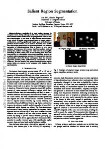
From Equation 19, it may be observed that vertices of the graph included in the dense subgraph set Sdense are given priority based on their degrees in the subgraph found. The map enhancement factor, γ (γ >1) in the final saliency map computation suppresses the saliency value of pixels in regions that correspond to nodes with low degrees. On the other hand, pixels corresponding to nodes with relatively high degrees, closer to the maximum degree in the dense subgraph set Gdense are assigned greater saliency values. A pixel corresponding to a node (a segmented region) not included in the dense subgraph set is assigned a value zero. Saliency value of a segmented region is directly proportional to the corresponding node degree. Therefore, saliency values of nodes with lower degrees than the mean degree, which contribute to non-salient regions, are suppressed and values of nodes with degrees higher than the mean degree, which contribute to salient regions, are enhanced. This ensures that sufficient contrast is generated in the saliency map and the salient regions may be easily distinguished from the non-salient portions. The variation of saliency values with varying node degrees is shown in Figure 7. The final saliency map, Mf inal is obtained after normalizing the map Mdense . Figure 6 depicts the flow of the proposed method in detailed steps. The graphs Gimage and GGBV S have been shown to be constructed by the multiplication of the respective feature, spatial and compactness edge-weights. 3.6. Multiple Salient Region Detection In this section, we demonstrate how multiple salient regions can be extracted using the proposed method. Figure 8(b) shows the graph GGBV S constructed from the input image in Figure 8(a). In the example shown, N = 44 is the total number of graph nodes, and the value of the parameter k = 28. The green colored nodes correspond to nodes with high degrees (degree ≥ 5). Procedure 1, which is a naive method, randomly selects 14 edges (k/2 = 14) and then includes the set of vertices incident with these edges, adding arbitrary vertices 14
Figure 6: Detailed steps in the proposed method.
Figure 7: Variation of assigned saliency values of pixels with varying node degrees. For the generated plot, mean of node degrees = 30.90 and γ = 3.
15
Figure 8: Multiple salient region extraction using k-dense subgraph algorithm. (a) Original image. (b) Graph, GGBV S (c) Multiple salient regions extracted after k-dense subgraph computation. (d) Final Saliency map, Mf inal .
to this set if its size is smaller than k (= 14). For procedure 2, the first fourteen (k/2 = 14) nodes (green colored) to be included in the dense subgraph set, are selected based on node degree values. The nodes with the highest number of neighbors in the already selected set of 14 nodes (marked in green), are the remaining nodes to be included in the 28-dense subgraph. Procedure 3 followed in the algorithm may also be analyzed along similar lines. This way, the vertex sets V S1 , V S2 and V S3 are formed from procedures 1, 2 and 3 respectively. We get the final dense subgraph (nodes and edges marked in red) in Figure 8(c) with 28 nodes as the densest among these three sets. This corresponds to three separate region clusters, which are detected as salient regions by the algorithm. Figure 8(d) shows the saliency map obtained by the dense subgraph computed in Figure 8(c). It may be noted here that, the nodes with high degrees are not localized in image space, as shown in the example. Correspondingly, the dense subgraph algorithm finds separate dense subgraphs at all image locations, where the node degrees are high. This property of the algorithm enables our model to detect multiple salient regions in an image effectively. 4. Experimental Results and Evaluation 4.1. Datasets We used the following datasets in our experiment. • Test datasets: – Single salient object dataset: We used images from the popular MSRA dataset [27], which is the largest object dataset containing 20,000 images in set A and 5,000 images in set B. Achanta [16] created a dataset 16
containing 1000 accurate object-contour based human-labeled ground truths corresponding to 1000 images selected from the set B of MSRA salient object dataset. We use the ASD dataset [16], created by Achanta as it enables easy quantitative evaluation. To evaluate our method on a slightly more complex dataset, we also use the PASCALS dataset for evaluation. The PASCAL-S dataset is derived from the validation set of PASCAL VOC 2010 [54] segmentation challenge and contains 850 natural images surrounded by complex background. – Multiple salient object dataset: To demonstrate the efficacy of our model to images with multiple salient objects, we tested the results on the SED2 dataset [26], as it contains 100 images, each with two salient objects. Pixelwise ground truth annotations for salient objects in all 100 images are provided. The CAS model [23] was not compared on this dataset, due to lack of author provided results or executable code. The results obtained by running the source codes of the methods (which are made available in their respective websites) or using author provided data, were used for comparison. • Validation dataset: There are two main parameters in the proposed method: – The k value in k-dense subgraph, which selects the participation of nodes in dense subgraph in determining the saliency values of regions, and – The map enhancement factor, γ, to adjust the quality of saliency maps. To choose these parameters, we used a small validation dataset consisting of 200 images randomly chosen from set A of MSRA dataset [27] and pixel accurate salient object labeling obtained from data used in [9]. 4.2. Experimental Setup We compared our model with eight other well known models, on the test dataset. These are: • Graph based saliency model (GB) [1](graph based) • Frequency tuned saliency model (FT)[16](frequency based) • Maximum Symmetric Surround saliency model (MSSS) [20](symmetric surround based) • Global contrast model (HC, RC) [9](region based) • Over-segmentation model (OS) [22](region segmentation based) • Contrast-Aware Saliency model (CAS) [23](region based) • Low rank matrix recovery model (LR) [24](region based) 17
Figure 9: Plot of F-measure value with k-value (used in dense k-subgraph algorithm) on validation dataset.
• Simple prior combination model (SDSP) [28](prior combination based) • Principle Component Analysis model (PCA) [46] (region based) • Graph based Manifold Ranking model (MR) [29] (graph based) We set the number of superpixel nodes, η = 250 for all test images, as discussed in section 3. As discussed in the previous section, we used set A of MSRA dataset [27] as the validation set to choose the parameters k and the map enhancement factor, γ. We calculated the F-measure values (as in Equation 20) on this validation set, for 0.1η ≤ k ≤ 1.0η (η being the total number of superpixels) and plotted the result as shown in Figure 9. k = 0.8η yielded the highest Fmeasure value (Fα = 0.614). The saliency maps with varying k values are shown in Figure 11. It may be observed that, saliency maps corresponding to k = 80%η, resemble the ground truth data better than other values of k. Unwanted image patches appear for other k values. For lower values of k, not all salient regions get detected and for higher values, unwanted background regions are labeled as salient regions. Similarly, we calculated the F-measure values for varying map enhancement factor, γ on this dataset, taking k = 0.8η. However, no significant improvement in F-measure values was observed with increasing γ. This is due to the fact that F-measure is based on binarized maps and non-salient regions with relatively low saliency values are still assigned zero value in the binarized map, as γ value is decreased. Figure 10 shows the impact of varying the value of γ on the generated saliency maps. We observe that salient regions become more prominent and stand out from the non-salient background portions with increasing γ value. However saliency maps cease to improve much with γ > 3. This observation led us to select γ = 3. Figures 12, 13 and 14 show the qualitative comparison of results obtained by the proposed method with other well known models considered in this paper. 18
Figure 10: Effect of varying map enhancement factor, γ on final saliency maps, Mf inal .
Figure 11: Saliency maps with varying k (k as in k-dense subgraph) values.
19
Figure 12: Comparison of saliency maps obtained by different methods on the ASD dataset [16]: (a) Original image, (b) GBVS model [1], (c) Frequency tuned model [16], (d) Maximum Symmetric Surround model [20], (e) Global contrast model (HC) [9], (f) Over-segmentation model [22], (g) Contrast-Aware Saliency model [23], (h) Low rank matrix model [24], (i) Simple prior combination model [28], (j) Principle component model [53], (k) Graph based manifold ranking model [29], (l) Our model and (m) Ground truth.
Figure 13: Comparison of saliency maps obtained by different models on the SED2 dataset [26]: (a) Original image, (b) GBVS model [1], (c) Frequency tuned model [16], (d) Maximum Symmetric Surround model [20], (e) Global contrast model (RC) [9], (f) Over-segmentation model [22], (g) Low rank matrix model [24], (h) Simple prior combination model [28], (i) Principle component model [53], (j) Graph based manifold ranking model [29], (k) Our model and (l) Ground truth.
20
Figure 14: Comparison of saliency maps obtained by different models on the PASCAL-S dataset [33]: (a) Original image, (b) GBVS model [1], (c) Frequency tuned model [16], (d) Maximum Symmetric Surround model [20], (e) Global contrast model (RC) [9], (f) Oversegmentation model [22], (g) Low rank matrix model [24], (h) Simple prior combination model [28], (i) Principle component model [53], (j) Graph based manifold ranking model [29], (k) Our model and (l) Ground truth.
Figure 15: Comparison of base method (GBVS) and proposed model. (a) Original image (b) GBVS saliency map (c) Saliency map, MGBV S (d) Final saliency map, Mf inal (e) Ground truth
21
Figure 15 compares the base model, GBVS [1] with the two stage saliency maps MGBV S and Mf inal we obtain in this paper. It may be observed that the blurred saliency maps of the GBVS algorithm get significant improvement after implementation of dense subgraph computation. Our model operates on image regions or superpixels and refines the region based GBVS algorithm as compared to base model [1], which operates at pixel level resulting in smooth transition from salient to non-salient portions (column (b)). Region compactness incorporated in the algorithm helps to preserve object boundaries, overcoming this limitation. The background image regions which get detected as salient by the region based GBVS algorithm (maps in column (c)) are eliminated to a great extent in the saliency maps (column (e)) refined by k-dense subgraph algorithm. 4.3. Evaluation metric The quantitative evaluation of the algorithm is carried out based on precision, recall, F-measure and Mean Absolute Error. Precision is a measure of accuracy and is calculated as ratio of number of pixels jointly predicted salient by binarized saliency map and ground truth image and the number of pixels predicted salient by the binarized saliency map. Recall is a measure of completeness and is calculated as the ratio of number of pixels jointly predicted salient by binarized saliency map and ground truth and the number of pixels predicted salient by the ground truth image. F-measure is an overall performance measurement indicator which is computed as the weighted harmonic mean between the precision and recall values. It is defined as: (1 + α) · P recision · Recall (20) α · P recision + Recall where the coefficient α is set to 1 to indicate equal importance of precision and recall. After normalizing the final saliency map, Mf inal to an 8-bit grayscale image, we threshold the map in the range Tf ∈ [0, 255], to get 256 binarized maps corresponding to each threshold value in this range. Different precision-recall pairs are obtained for each of the 256 maps, and a precision-recall curve is drawn. The average precision-recall curves are generated by averaging the results from all the 1000 test images from the ASD dataset [16] (in Figure 16(a)), 100 images from the SED2 dataset (in Figure 16(b)) and 850 images from the PASCAL-S dataset (in Figure 16(c)) respectively. Furthermore, to evaluate the applicability of saliency maps for salient object detection more explicitly, we used an image dependent adaptive threshold (Ta ) to segment objects in the image, as followed in [16]. A fixed threshold value in standard thresholding technique, does not always correctly demarcate the salient region from the background. Adaptive thresholding overcomes this limitation. We set the threshold Ta as twice the mean saliency value of the saliency map. Using this adaptive threshold, we obtain the binarized versions of the saliency maps, for all models. The binarized saliency maps are then compared to the ground truth images to compute the metrics of precision, recall, and F-measure for all models compared, as shown in Fα =
22
(a)
(b)
(c) Figure 16: Comparison of precision-recall curves of compared models on (a) ASD dataset [16] (b) SED2 dataset [26] (c) PASCAL-S dataset [33]. (GB: GBVS method [1], FT: Frequency tuned model [16], MSSS: Maximum Symmetric Surround model [20], HC, RC: Global contrast model [9], OS: Over-segmentation model [22], CAS: Contrast-Aware model [23], LR: Low rank matrix model [24], SDSP: Simple prior combination model [28], PCA: Principle component model [53], MR: Graph based manifold ranking model [29], Proposed: Our method.)
23
Figure 17. These metrics are first computed on all the test images individually and then averaged over the whole dataset to obtain the overall performance in terms of average precision-recall curve and overall F-measure. As neither precision nor recall measures consider the number of pixels correctly marked as non-salient (i.e true negative saliency assignments), we follow Perazzi et al. [25] to evaluate the Mean Absolute Error (MAE) for the models compared. MAE between an unbinarized saliency map S and the binary ground truth G for all image pixels IP is calculated as in Equation 21. M AE =
1 X |S(IP ) − G(IP )|, |I|
(21)
P
where, |I| is the number of image pixels. For all methods, we considered the final saliency maps and compared them to the binary ground truth data to obtain the average MAE on the used dataset. Results of average MAE evaluation on compared methods have been shown in Figure 18. 4.4. Evaluation Quantitative evaluation From Figure 17, it is clear that the proposed method scores generally higher precision, recall and F-measure than previously proposed methods used for comparison. The MR method [29] scores better in terms of precision rate as compared to our model on all three datasets, but our method outperforms it in terms of recall rate and overall F-measure value. On the PASCAL-S dataset [33], the RC [20] and the SDSP [28] methods also have a slight edge over our method in terms of precision rate, but their recall rates and overall F-measure values are significantly lower than that of the proposed method. It is observed that our algorithm, in general, achieves better recall values than precision. A high recall value of an algorithm indicates that most of the relevant results are detected by it. In an experiment conducted in [55], it was found that object region based saliency models can easily yield high precision values. However, a high recall value is generally achieved only by conducting the object segmentation operations either before or after the saliency computation. The high recall values of the algorithm thus helps our model to yield high quality object segmentations. Objectness estimation is another major application of a high recall saliency detection algorithm. Objectness is generally measured by constructing a small set of bounding boxes to improve efficiency of the classical sliding window pipeline. High recall at such a set of bounding box proposals is often a major target. Average MAE, which provides a better estimate of dissimilarity between the saliency map and ground truth (as evaluated in Figure 18), shows that our method outperforms the existing models by a fair margin, for all the three datasets. The MR method [29] performs comparable to our method on the ASD [16] and the PASCAL-S [33] datasets. On the SED2 dataset [26] however, average MAE of the RC method [9] is most comparable to our method. 24
(a)
(b)
(c) Figure 17: Precision, recall, and F-measure value histogram of the different models on (a) ASD dataset [16] (b) SED2 dataset [26] (c) PASCAL-S dataset. (GB: GBVS method [1], FT: Frequency tuned model [16], MSSS: Maximum Symmetric Surround model [20], HC, RC: Global contrast model [9], OS: Over-segmentation model [22], CAS: Contrast-Aware model [23], LR: Low rank matrix model [24], SDSP: Simple prior combination model [28], PCA: Principle component model [53], MR: Graph based manifold ranking model [29], Proposed: Our method.) 25
(a)
(b)
(c) Figure 18: Average MAE of the different models on (a) ASD dataset [16] (b) SED2 dataset [26] (c) PASCAL-S dataset [33]. (GB: GBVS method [1], FT: Frequency tuned model [16], MSSS: Maximum Symmetric Surround model [20], HC, RC: Global contrast model [9], OS: Over-segmentation model [22], CAS: Contrast-Aware model [23], LR: Low rank matrix model [24], SDSP: Simple prior combination model [28], PCA: Principle component model [53], MR: Graph based manifold ranking model [29], Proposed: Our model.)
26
The method proposed is based on the graph based visual saliency model (GB [1]) upon which it improvises to extract salient regions using a graph theoretic model. There is a significant rise in F-measure value as compared to the GB model (24.5% i.e from 63.1% to 87.6% on the ASD dataset [16], 23.5% i.e from 45.4% to 68.9% on the SED2 dataset [26] and 21.4% i.e from 37.3% to 58.7% on the PASCAL-S dataset [33]). Qualitative evaluation From the qualitative comparison in Figure 12, it is observed that models in columns (e) and (h) yield saliency maps with sufficient contrast between salient and non-salient regions, however background regions are still highlighted. On the other hand, the over-segmentation model [22] (column (f)) generates low contrast maps and thus not suitable for object segmentation. The saliency maps generated by the MR method [29] generally have nice contrast. However, undesired background regions are highlighted for some images, such as in rows 5 and 7 or incomplete saliency detection is observed such as in row 4. The proposed model generates saliency maps which are quite similar to the desired results of salient object segmentation. The salient regions get more uniformly highlighted with proper suppression of the background regions, as compared to the other methods. In Figure 13, similar observations may be made regarding object shape retention of multiple objects in our saliency maps, in column (h), though the method fails for the image in row 7, due to prominence of background region. The global contrast model [9] (column (e)) generates comparable maps, however for some images does not highlight multiple objects as salient, as may be observed in row 6 (only the right cow is highlighted). Similarly, the MR method [29] fails to highlight the left cow (in row 6) and the left shell (in row 5). For the PASCAL-S dataset [33] (Figure 14), our method clearly highlights the salient regions better than other models. For instance, in rows 3 and 6, almost all other methods fail to clearly demarcate the entire salient image region or stress inadequate image portions as being salient, as in row 2 (only bird neck has more saliency value). Our saliency model suppresses the non-salient regions effectively and generates high-resolution saliency maps with well preserved shape information due to the compactness factor incorporated in the algorithm. Thus it is inherently advantageous for object segmentation tasks. 4.5. Computational cost In addition to the saliency prediction accuracy, we compare the execution time of different methods. The computational cost of the compared methods on a 2.39 GHZ Intel(R) Core i3 CPU with 4GB RAM, are summarized in Table 1. The software platform was Matlab R2013a. Table 1 shows the average execution time taken by each saliency detection method for processing an image on the SED2 dataset [26]. The computational costs of different saliency detection methods vary greatly, as seen from Table 1. The proposed method has lesser execution time than the LR [24], PCA [53] and CAS [23] methods. Other methods run faster than the proposed method, but their saliency detection accuracies are quite lower than the method proposed as evident from section 4.4. 27
Method Time (in sec.) Method Time (in sec.)
GB [1] 1.58 LR [24] 25.18
FT [16] 0.09 SDSP [28] 0.26
MSSS [20] 0.95 PCA [53] 11.56
RC [9] 0.23 MR [29] 0.26
OS [22] 3.86 Proposed 6.42
CAS [23] 6.63
Table 1: Average execution time of each method on the SED2 dataset [26].
4.6. Failure Cases and Analysis As shown in the previous section, the proposed model outperforms the compared saliency models on both qualitative and quantitative evaluation. However, some difficult images are still challenging for the model proposed as well as other compared models. If an image contains a part of background regions, which are visually salient against the major part of background such as row 8 in Figure 12 and rows 6 and 7 in Figure 13, the salient object is not properly highlighted or the nearby background regions are erroneously highlighted in the generated saliency maps. The proposed model, as well as other compared saliency models, are yet to be effective to handle such challenging cases. Also as the proposed algorithm uses intensity, color, and compact features to determine saliency, it may fail to detect irregular shape in a visual information scene, since all objects have the same intensity/color and similar compactness values. 5. Conclusion and Future Work In this article, we have presented a new method for salient region detection. The proposed method takes the saliency results of the previously proposed graph based saliency detection method, applies it on segmented image found by the SLIC superpixel segmentation algorithm and introduces the k-dense subgraph finding problem to that of saliency detection to improve the extraction of salient parts in a visual information scene. Future research scope by this approach may include implementing better dense subgraph finding algorithms and selection of features used to construct graph. The method proposed is based on global image features only. Local image features and contrast information, if considered in future work, may further enhance the salient region detection ability of the algorithm proposed. Shape and orientation information can also be included as a feature to address the issues of irregular shape detection. We will attempt to incorporate these changes and also generalize the proposed work in video saliency detection, in our future work. However, based on the experiments using image data sets labeled with ground truth salient region, the method followed here has been shown to provide better region based saliency maps as compared to ten well known saliency detection methods and is capable of segmenting objects from an image effectively.
28
References [1] J. Harel, C. Koch, and P. Perona, “Graph-based visual saliency,” in Proc. Adv. Neural Inf. Process. Syst., pp. 545–552, 2006. [2] R. Pal, A. Mukherjee, P. Mitra and J. Mukherjee, “Modeling visual saliency using degree centrality,” IET Computer Vision, vol. 4, no. 3, pp. 218-229, Sep. 2010. [3] L. Itti, C. Koch, and E. Niebur, “A model of saliency-based visual attention for rapid scene analysis,” IEEE Trans. Pattern Anal. Mach. Intell., vol. 20, no. 11, pp. 1254–1259, Nov. 1998. [4] U. Feige, G. Kortsarz and D. Peleg, “The Dense k-Subgraph Problem,” Algorithmica, vol. 29, pp. 2001, 1999. [5] Y. Sun and R. Fisher, “Object-based attention for computer vision,” Artif. Intell., vol. 146, no. 1, pp. 77–123, 2003. [6] J. Duncan, “Selective attention and the organization of visual information,” J. Exp. Psychol. Gen., vol. 113, no. 4, pp. 501–517, 1984. [7] M. Z. Aziz and B. Mertsching, “Fast and robust generation of feature maps for region-based visual attention,” IEEE Trans. Image Processing, vol. 17, no. 5, pp. 633–644, May 2008. [8] T. Avraham and M. Lindenbaum, “Esaliency (extended saliency): Meaningful attention using stochastic image modeling,” IEEE Trans. Pattern Anal. Mach. Intell., vol. 32, no. 4, pp. 693–708, Apr. 2010. [9] M.-M. Cheng, G.-X. Zhang, N. J. Mitra, X. Huang, and S.-M. Hu, “Global contrast based salient region detection,” in Proc. IEEE Int. Conf. Comput. Vision Pattern Recognit., pp. 409–416, Jun. 2011. [10] G. Boccignone and M. Ferraro, “Modeling gaze shift as a constrained random walk,” Physica A, vol. 331, no. 1, pp. 207–218, 2004. [11] L. F. Costa. (2007). Visual Saliency Random Walks on Complex Networks http://arxiv.org/abs/physics/0603025v2
and Attention as [Online]. Available:
[12] V. Gopalakrishnan, Y. Hu, and D. Rajan, “Random walks on graphs for salient object detection in images,” IEEE Trans. Image Processing, vol. 19, no. 12, pp. 3232–3242, Dec. 2010. [13] V. Gopalakrishnan, Y. Hu, and D. Rajan, “Random walks on graphs to model saliency in images,” in Proc. IEEE Int. Conf. Comput. Vision Pattern Recognit., pp. 1698–1705, Jun. 2009.
29
[14] W. Wang, Y. Wang, Q. Huang, and W. Gao, “Measuring visual saliency by site entropy rate,” in Proc. IEEE Int. Conf. Comput. Vision Pattern Recognit., pp. 2368–2375, Jun. 2010. [15] D. Walther and C. Koch, “Modeling attention to salient proto-objects,” Neural Netw., vol. 19, no. 9, pp. 1395–1407, 2006. [16] R. Achanta, S. Hemami, F. Estrada, and S. Susstrunk, “Frequency-tuned salient region detection,” in Proc. IEEE Int. Conf. Comput. Vision Pattern Recognit., pp. 1597–1604, 2009. [17] C. W. H Ngau, L. M. Ang, and K. P. Seng, “Comparison of color spaces for visual saliency,” in Proc. Int. Conf. Intellig. Human Mach. Systems and Cybernetics, pp. 278-281, 2009. [18] J. S. Kim, J. Y. Sim and C. S. Kim, “Multiscale Saliency Detection Using Random Walk with Restart,” IEEE Trans. Circuits Syst. Video Techn., vol 24, no. 2, pp. 198-210, Feb. 2014. [19] R. Achanta, A. Shaji , K. Smith, A. Lucchi, P. Fua and S. Susstrunk, “SLIC Superpixels Compared to State-of-the-Art Superpixel Methods,” IEEE Trans. Pattern Anal. Mach. Intell., vol 34, no. 11, pp. 2274 - 2282, May. 2012. [20] R. Achanta and S. Susstrunk, “Saliency Detection using Maximum Symmetric Surround,” in Proc. IEEE Int. Conf. Image Processing, 2010. [21] S. P. Lloyd, “Least squares quantization in PCM,” IEEE Trans. Inform. Theory, vol. 28, no. 2, pp. 129–137, Mar. 1982. [22] X. Zhang, Z. Ren, D. Rajan and Y. Hu, “Salient Object Detection through Over-Segmentation,” in IEEE Int. Conf. Multimedia and Expo, Melbourne, 2012. [23] H. H. Yeh and C.-S. Chen, “From Rareness To Compactness: ContrastAware Image Saliency Detection,” in Proc. IEEE Int. Conf. Image Processing, Orlando, Florida, USA, 2012. [24] X. Shen and Y. Wu, “A unified approach to salient object detection via low rank matrix recovery,” in Proc. IEEE Int. Conf. Comput. Vision Pattern Recognit., 2012. [25] F. Perazzi, P. Krahenbuhl, Y. Pritch, and A. Hornung, “Saliency filters: Contrast based filtering for salient region detection,” in Proc. IEEE Int. Conf. Comput. Vision Pattern Recognit., pp. 733–740, 2012. [26] S. Alpert, M. Galun, R. Basri, and A. Brandt, “Image segmentation by probabilistic bottom-up aggregation and cue integration,” in Proc. IEEE Int. Conf. Comput. Vision Pattern Recognit., Jun. 2007, pp. 1–8.
30
[27] T. Liu, Z. Yuan, J. Sun, J. Wang, N. Zheng, T. X., and S. H.Y., “Learning to detect a salient object,” IEEE Trans. Pattern Anal. Mach. Intell., vol 33, no. 2, pp. 353 - 367, 2011. [28] L. Zhang, Z. Gu and H. Li, “SDSP: A novel saliency detection method by combining simple priors,” in Proc. IEEE Int. Conf. on Image Processing, Melbourne, 2013. [29] C. Yang, L. Zhang, H. Lu, X. Ruan and M-H Yang, “Saliency Detection via Graph-Based Manifold Ranking,” in Proc. IEEE Int. Conf. Comput. Vision Pattern Recognit., pp. 3166-3173, 2013. [30] B. Jiang, L. Zhang, H. Lu, C. Yang and M-H Yang, “Saliency Detection via Absorbing Markov Chain,” in IEEE Int. Conf. on Computer Vision (ICCV), pp. 1665 - 1672, 2013. [31] O. Boiman and M. Irani, “Detecting irregularities in images and in video,” International Journal of Computer Vision, 74(1), pp. 17–31, 2007. [32] L. Changyang, Y. Yuan, W. Cai, Y. Xia and D. D. Feng, “Robust Saliency Detection via Regularized Random Walk Ranking,” in Proc. IEEE Int. Conf. Comput. Vision Pattern Recognit., 2015. [33] Y. Li, X. Hou, C. Koch, J. Rehg, and A. Yuille, “The secrets of salient object segmentation.” in Proc. IEEE Int. Conf. Comput. Vision Pattern Recognit., 2014. [34] Y. Qin, H. Lu, Y. Xu and H. Wang, “Saliency Detection via Cellular Automata,” in Proc. IEEE Int. Conf. Comput. Vision Pattern Recognit., 2015. [35] M.G. Albanesi, M. Ferretti and F. Guerrini, “Adaptive image compression based on regions of interest and a modified contrast sensitivity function” in 15th International Conference on Pattern Recognition, 2000. [36] J. Shao, J. Gao and J. Yang, “Synergetic Object Recognition Based on Visual Attention Saliency Map” in IEEE Int. Conf. on Information Acquisition, pp. 660 - 665, 2006. [37] P.-E. Forssen, D. Meger, K. Lai, S. Helmer, J.J. Little and D.G. Lowe, “Informed visual search: Combining attention and object recognition” in IEEE Int. Conf. on Robotics and Automation, pp. 935 - 942, 2008. [38] H. Nakano, S.Okuma and Y. Yano, “A study on fast object recognition based on selective visual attention system” in IEEE Int. Conf. on Systems, Man and Cybernetics, pp. 2116 - 2121, 2008. [39] C. Siagian and L. Itti, “Rapid Biologically-Inspired Scene Classification Using Features Shared with Visual Attention,” in IEEE Trans. Pattern Anal. Mach. Intell., vol 29, no. 2, pp. 300 - 312, 2007.
31
[40] N. D. B. Bruce, J. K. Tsotsos, “Saliency, attention, and visual search: An information theoretic approach” in Journal of Vision, vol 9, issue (3):5, pp. 1–24, 2009. [41] D. A. Klein and S. Frintrop, “Center-surround Divergence of Feature Statistics for Salient Object Detection” in IEEE Int. Conf. on Computer Vision (ICCV), 2011. [42] X. Hou, J. Harel, and C. Koch, “Image Signature: Highlighting Sparse Salient Regions” in IEEE Trans. Pattern Anal. Mach. Intell., vol 34, no 1, Jan. 2012. [43] R. Zhao, W. Ouyang, H. Li and X. Wang, “Saliency Detection by MultiContext Deep Learning” in Proc. IEEE Int. Conf. Comput. Vision Pattern Recognit., 2015. [44] A. M. Treisman and G. Gelade, “A feature integration theory of attention,” Cognitive Psychology, 12, pp. 97–136, 1980. [45] C. Koch and S. Ullman, “Shifts in selective visual attention: towards the underlying neural circuitry,” Human Neurobiology, 4(4), pp. 219–227, 1985. [46] B. Schauerte and R. Stiefelhagen, “Quaternion-based spectral saliency detection for eye fixation prediction,” in European Conference On Computer Vision, 2012. [47] A. Borji and L. Itti, “State-of-the-Art in Visual Attention Modeling” IEEE Trans. Pattern Anal. Mach. Intell., vol 35, no. 1, Jan. 2013. [48] B. Alexe, T. Deselaers, and V. Ferrari. “What is an object?” in Proc. IEEE Int. Conf. Comput. Vision Pattern Recognit., 2010. [49] T. Liu, Z. Yuan, J. Sun, J. Wang, N. Zheng, X. Tang, and H.-Y. Shum. “Learning to detect a salient object.” IEEE Trans. Pattern Anal. Mach. Intell., 2009. [50] L. Itti and P. Baldi, “Bayesian surprise attracts human attention,” Vision Research, 49(10), 2009. [51] L. Zhang, M. H. Tong, T. K. Marks, H. Shan, and G. W. Cottrell, “Sun: A bayesian framework for saliency using natural statistics,” Journal of Vision, 8(32), 2008. [52] J. R. Norris, “Markov Chains” Cambridge, U.K.: Cambridge University Press, 1997. [53] R. Margolin, L. Zelnik-Manor and A. Tal, “What Makes a Patch Distinct” in Proc. IEEE Int. Conf. Comput. Vision Pattern Recognit., 2013.
32
[54] M. Everingham, L. Van Gool, C. K. Williams, J. Winn and A. Zisserman, “The pascal visual object classes (voc) challenge,” International journal of computer vision, 88(2), pp. 303– 338, 2010. [55] J. Li and W. Gao, “Visual Saliency Computation: A Machine Learning Perspective,” Springer Publishing Company, Incorporated, 2014.
33