A Compact Genetic Algorithm for the Network Coding Based ...

Title: A Compact Genetic Algorithm for the Network Coding Based Resource Minimization Problem Authors: Huanlai Xing (corresponding author), Rong Qu Affiliation: The Automated Scheduling, Optimisation and Planning (ASAP) Group, School of Computer Science, The University of Nottingham Address: School of Computer Science, University of Nottingham, Nottingham, NG8 1BB, United Kingdom Phone: +44-0115 84 66554 Email: [email protected]; [email protected]

Abstract: In network coding based data transmission, intermediate nodes in the network are allowed to perform mathematical operations to recombine (code) data packets received from different incoming links. Such coding operations incur additional computational overhead and consume public resources such as buffering and computational resource within the network. Therefore, the amount of coding operations is expected to be minimized so that more public resources are left for other network applications. In this paper, we investigate the newly emerged problem of minimizing the amount of coding operations required in network coding based multicast. To this end, we develop the first elitismbased compact genetic algorithm (cGA) to the problem concerned, with three extensions to improve the algorithm performance. First, we make use of an all-one vector to guide the probability vector (PV) in cGA towards feasible individuals. Second, we embed a PV restart scheme into the cGA where the PV is reset to a previously recorded value when no improvement can be obtained within a given number of consecutive generations. Third, we design a problemspecific local search operator that improves each feasible solution obtained by the cGA. Experimental results demonstrate that all the adopted improvement schemes contribute to an enhanced performance of our cGA. In addition, the proposed cGA is superior to some existing evolutionary algorithms in terms of both exploration and exploitation simultaneously in reduced computational time.

Keywords: compact genetic algorithm; estimation of distribution algorithm; multicast; network coding

1

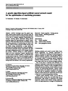
1. Introduction Network coding represents a generalized routing scheme in communications, and has been attracting increasing research attention in both information theory and computer science since its introduction in 2000 [1]. As a newly emerged paradigm, it brings a lot of benefits to communication networks in terms of increased throughput, balanced network payload, energy saving, security, robustness against link failures, and so on [2-7]. Instead of simply replicating and forwarding data packets at the network layer, network coding allows any intermediate node (i.e. router), if necessary, to perform arbitrary mathematical operations to recombine (i.e. code) data packets received from different incoming links. By doing so, the maximized multicast throughput bounded by the MAXFLOW MIN-CUT theorem can always be obtained [2]. Fig.1 shows an example of the superiority of network coding over traditional routing in terms of the maximum multicast throughput achieved [8]. In the network of 7 nodes and 9 links in Fig.1(a), s is the single source, and y and z are two sinks. Each direct link has a capacity of one bit per time unit. According to the MAX-FLOW MIN-CUT theorem, we know that the minimum cut Cmin between s and y (or between s and z) is two bits per time unit, so is the maximum multicast throughput from s to y and z. However, only 1.5 bits per time unit can be achieved as the multicast throughput if traditional routing is used. This is because link wx could only forward one bit (a or b) at a time to node x, and thus y and z cannot simultaneously receive two bits, as indicated in Fig.1(b). In Fig.1(c) where network coding is applied, node w is allowed to recombine the two bits it receives from t and u into one bit a b (symbol

here represents the Exclusive-OR

operation) and to output a b to node x. In this way, y and z are able to receive {a, a b} and {b, a b} respectively, and thus two bits information is available at each sink. Meanwhile, by calculating a (a b) and b (a b), y and z can then recover b and a, respectively. Insert Fig.1 somewhere here. In most of the previous research in network coding, coding is performed at all coding-possible nodes. However, to obtain an expected multicast throughput, coding may only be necessary at a subset of those nodes [9-11]. Fig.2 illustrates 2

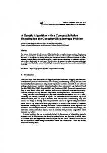
two network-coding-based data transmission schemes that could both achieve the maximum multicast throughput. Source s expects to transmit two bits (a and b) to four sinks, t1, t2, t3 and t4. Scheme A adopts two coding-possible nodes, namely node m and node n, as shown in Fig.2(a). Nevertheless, the same throughput can also be obtained by scheme B in Fig.2(b), where coding only occurs at node m. Due to the mathematical operations involved, network coding not only incurs additional cost such as computational overhead and transmission delay, but also consumes public resources, e.g. buffering and computational resources [12]. It is therefore important that the number of coding operations is kept minimized while the benefits of network coding are warranted. Unfortunately, this problem is NPhard [9-11]. Insert Fig.2 somewhere here. Although a large amount of research has been conducted on multicast routing problems by using advanced algorithms including evolutionary algorithms and local search based algorithms [13-17], a limited number of algorithms have been proposed in the literature of network coding based multicast. Most of these algorithms are based on either greedy methods or evolutionary algorithms. Langberg et al [12] and Fragouli et al [18] proposed different network decomposition methods and two greedy algorithms to minimize coding operations. However, the optimization of these algorithms depends on the traversing order of links. An inappropriate link traversal order leads to a deteriorated performance. Kim et al investigated evolutionary approaches to minimize the required network coding resources [9-11]. In [9], a genetic algorithm (GA) working in an algebraic framework has been put forward. However, it is applied to acyclic networks only. This has been extended to a distributed GA to significantly reduce the computational time in [10]. In [11], the authors compare and analyse GAs with two different genotype encoding approaches, i.e. the binary link state (BLS) and the binary transmission state (BTS). Simulations show that compared to BLS encoding, BTS encoding has much smaller solution space and leads to better solutions. Besides, their GA-based algorithms perform outstandingly better than the two greedy algorithms in [12] and [18] in terms of the best solutions achieved. Nevertheless, as we observed in our present work, GAs (e.g. [11]) have still shown to be weak in global exploration, even though a greedy sweep operator follows the evolution to further 3

improve the best individual. In our previous work [8], an improved quantuminspired evolutionary algorithm (QEA) has been developed to minimize the amount of coding operations. Simulation results demonstrate that the QEA outperforms simple GAs in many aspects including fast convergence. However, we observe in this paper that the improved QEA sometimes finds decent solutions at the cost of additional computational time. Recently, we also put forward a population based incremental learning (PBIL) to find the optimal amount of coding operations [19]. However, its main concern is how to apply network coding in delay sensitive applications. An extended compact genetic algorithm has thus been developed in this work to solve the highly constrained problems being concerned. As one of estimation of distribution algorithms (EDA) [20-22], the compact genetic algorithm (cGA) was first introduced in 1999 by Harik et al [23]. Whereas the simple genetic algorithm (sGA) maintains a population of solutions, cGA simply employs a probability vector (PV) while still retaining the order-one behavior (i.e. problem can be solved to optimality by combining only order-one schemata [23]) of the sGA with a uniform crossover. Contrary to sGA, cGA is much faster and efficient, and requires far less memory so that significant amounts of computational time and memory are saved. Hence, cGA has drawn an increasing research attention and been successfully applied to a number of optimization problems including evolvable hardware implementation [24-25], multi-FPGA partitioning [26], image recognition [27], TSK-type fuzzy model [28] and so on. Unfortunately, cGA is not always powerful, especially to complex optimization problems, due to the assumption that variables in any given problem are independent [29]. In this paper, we investigate the first elitism-based cGA to the minimization problem of coding operations in network coding based multicast. In our cGA, three novel schemes have been developed to improve the optimization performance of cGA. The first scheme is to, by using an all-one vector, adjust the PV in such a way that feasible individuals appear with higher probabilities. This scheme not only warrantees the cGA with a feasible elite individual at the beginning of evolution but also allows the PV to generate feasible individuals with increasingly higher probabilities. The second scheme is a PV restart scheme to reset the PV when the solution found cannot be improved within a given 4

number of consecutive generations. This scheme stops ineffective evolution and helps to increase the chance to hit an optimal solution. In the third scheme, a local search operator is devised to exploit the neighborhood of each feasible solution so that the local exploitation of our cGA is, to a large extent, enhanced. Simulation experiments have been conducted over a number of fixed and randomly generated multicast scenarios. Results demonstrate that all the adopted schemes are effective and the proposed cGA outperforms existing evolutionary algorithms in obtaining optimal solutions within reduced computational time.

2. Problem Description A communication network can be modeled as a directed graph G = (V, E), where V and E denote the set of nodes and links, respectively [2]. A single-source network coding based multicast scenario can be defined as a 4-tuple set (G, s, T, R), where the information needs to be transmitted at the data rate R from the source node s V to a set of sinks T = {t1,…,td} V in the graph G (V, E). The data rate R (a capacity of R units) is achievable if there is a transmission scheme that enables each sink tk, k = 1,…,d, to receive the information at the data rate R [911]. We assume each link has a unit capacity, and a path from s to tk thus has a unit capacity. If we manage to set up R link-disjoint paths {P1(s, tk),…,PR(s, tk)} from s to each sink tk T, we make the data rate R achievable. In this work we consider the linear network coding scheme which is sufficient for multicast applications [2]. In this paper, a subgraph in G is called a network coding based multicast subgraph (NCM subgraph, denoted by GNCM(s, T)) if there are R link-disjoint paths Pi(s, tk), i = 1,…,R, from s to each sink tk, k = 1,…,d, in this subgraph. An intermediate node nc is called a coding node if it performs a coding operation. Each coding node has at least one outgoing link, called coding link, if this link outputs the coded information. Take data transmission scheme in Fig.1(c) as an example, its NCM subgraph and the paths that make up of this subgraph are shown in Fig.3. The NCM subgraph is composed of four paths, i.e. P1(s, y), P2(s, y), P1(s, z) and P2(s, z), where paths to the same sink are link-disjoint. As we know, no coding is necessary at any intermediate node with only one incoming link. We refer to each non-sink node with multiple incoming links as a merging node which can perform coding [10-11]. We also refer to each outgoing link of a 5

merging node as a potential coding link. To determine if a potential coding link of a merging node becomes a coding link, we just need to check if the information via this link is dependent on a number of incoming links of the merging node. Insert Fig.3 somewhere here. For a given multicast scenario (G, s, T, R), the number of coding links, rather than coding nodes, is more precise to indicate the total amount of coding operations [12]. We therefore investigate how to construct a NCM subgraph GNCM(s, T) with the minimal number of coding links while achieving the expected data rate. We define the following notations: vij: a variable associated with the j-th outgoing link of the i-th merging node, i = 1,…,M, j = 1,…,Zi, where M is the total number of merging nodes and the i-th merging node has Zi outgoing links. vij = 1 if the j-th outgoing link of the i-th node serves as a coding link; vij = 0 otherwise. ncl(GNCM(s,T)) : the number of coding links in a constructed NCM subgraph GNCM(s,T). R(s, tk) : the achievable rate from s to tk. R: the defined data rate (an integer) at which s expects to transmit information. Pi(s, tk) : the i-th established path from s to tk, i = 1,…,R in GNCM(s, T). Wi(s, tk) : the set of links of Pi(s, tk), i.e. Wi(s, tk) = {e | e Pi(s, tk)}. Based on the above notations, we define in this paper the problem of network coding based resource minimization as to minimize the number of coding links while achieving a desired multicast throughput, shown as follows: Zi

M

Minimize: ncl (GNCM (s, T ))

vij i 1 j 1

Subject to: R(s, tk)

R,

tk T

(1) (2)

R

 W ( s, t i

i 1

k

)

,

tk

T

(3)

Objective (1) defines our problem as to minimize the number of coding links in the constructed NCM subgraph; Constraint (2) defines that the achievable data rate from s to each sink must be at least R so that we can set up R paths for each sink; Constraint (3) indicates that for an arbitrary tk the R constructed paths Pi(s, 6

tk), i = 1,…,R, must have no common link so that each sink can receive information at rate R.

3. An Overview of Compact Genetic Algorithm cGA is a variant of EDA, where its population is implicitly represented by a real-valued probability vector (PV). At each generation, only two individuals are sampled from the PV and a single tournament is performed between them, i.e. a winner and a loser are identified [23]. The PV is then adjusted and shifted towards the winner. As the cGA evolves, the PV converges to an explicit solution. We denote the aforementioned PV at generation t by P(t) = {P1t,…,PLt}, where L is the length of each individual (see more details in section 4). The value at each locus of P(t), i.e. Pit, i = 1,…,L, is initialized as 0.5 so that initially all solutions in the search space appear with the same probability. Let winner(i) and loser(i), i = 1,…,L, be the i-th bit of the winner and the loser, respectively, and 1/N be the increment of the probability of the winning alleles after each competition between the winner and the loser, where N is an integer. Note that although cGA produces two individuals at each generation, it can mimic the convergence behavior of a sGA with a population size N [23]. The procedure of the standard cGA is presented in Fig.4. Insert Fig.4 somewhere here. In this paper, the proposed cGA is based on the persistent elitist cGA (pecGA) introduced in [29]. Compared with the standard cGA, the procedure of pecGA is almost the same except the two steps, i.e. steps 6 and 7, in Fig.4. Fig.5 illustrates steps 6 and 7 in pe-cGA [29], where two individuals are created at generation t = 1. In the following generations, only one new individual is created to compete with the winner from previous generations. The winner (the elite individual), on the other hand, is never changed as long as no better individual has been sampled from the PV. Insert Fig.5 somewhere here.

7

4. The Proposed Compact Genetic Algorithm In this section, we first describe the individual representation and the fitness evaluation in our proposed cGA, based on which all the aforementioned improvement schemes are devised. 4.1 Individual Representation and Fitness Evaluation Encoding represents one of the most important key issues in designing efficient and effective evolutionary algorithms in many complex optimization problems, including the newly emerged coding resource minimization problem concerned in our work. To cater for the complex network structure in the problem studied here, we adopt the Graph Decomposition Method in [10-11] to represent solutions and calculate the fitness of each individual in the cGA. To detect the number of coding operations at each merging node in a given network topology G, a secondary graph GD is created by decomposing each merging node in G into a number of nodes connected with additional links introduced. For the i-th merging node with In(i) incoming links and Out(i) outgoing links, In(i) nodes, u1,…,uIn(i), referred to as incoming auxiliary nodes, and Out(i) nodes, w1,…,wOut(i), referred to as outgoing auxiliary nodes, are created. The original i-th merging node can thus be seen as decomposed into two sets of nodes. The j-th incoming link of the i-th original merging node is redirected to node uj; and the k-th outgoing link of the i-th merging node is redirected to node wk. Besides, a directed link e(uj, wk) is inserted between each pair of nodes (uj, wk), j = 1,…,In(i), k = 1,…,Out(i). In our cGA, we associate each binary bit of an individual X with one of the newly introduced links between those auxiliary nodes, e.g. e(uj, wk) in GD. A value ‘1’ at a bit in X means its corresponding link exists in GD, ‘0’ otherwise. Each individual therefore corresponds to an explicit secondary graph GD which may or may not provide a valid network coding based routing solution. To evaluate a given individual X, we first check if X is feasible. For each sink tk, k = 1,…,d, we use the Goldberg algorithm [30], a classical max-flow algorithm, to compute the max-flow between the source s and tk in the corresponding GD of X. As mentioned in section 2, each link in G has a unit capacity. The max-flow between s and tk is thus equivalent to the number of link-disjoint paths found by the Goldberg algorithm between s and tk. If all d max-flows are at least R, rate R is 8

achievable and the individual X is feasible. Otherwise, the individual X is infeasible. For each infeasible individual X, we set a sufficiently large fitness value Ψ to its fitness f(X) (in this paper, Ψ = 50). If X is feasible, we first determine its corresponding NCM subgraph GNCM(s, T) and then calculate its fitness value. For each sink tk T, we select R paths from the obtained link-disjoint paths from s to tk (if the max-flow is R then we select all the link-disjoint paths), and therefore obtain in total R·d paths, e.g. Pi(s, tj), i = 1,…,R, j = 1,…,d. We map all the selected paths to GD and obtain a GNCM(s, T) in which coding operations occur at the outgoing auxiliary nodes with two or more incoming links. The fitness value f(X) can then be set to the number of coding links in the GNCM(s, T). Note that our fitness evaluation is slightly different from the one in [10-11] where authors only concern if the subgraph obtained can meet the data rate requirement, i.e. each constructed subgraph in [10-11] potentially offers a data rate larger than required because the subgraph may have more link-disjoint paths than expected from the source to the sink. Our NCM subgraph provides the exact expected data rate, and thus is more likely to occupy less link and coding resources. 4.2 The Use of an All-one Vector The problem concerned in our work is highly constrained within complex network structures, and thus infeasible solutions form a large proportion of the solution space. The PV hence may not be able to efficiently evolve with a limited number of feasible individuals, i.e. the optimization of cGA could be seriously weakened due to the lack of feasible individuals. Kim et al [10-11] noticed this problem and inserted an all-one vector, i.e. ‘11…1’, into the initial population to warrantee that their GAs start with at least one feasible individual (the all-one vector ensures that all newly introduced links exist in GD and guarantees a feasible NCM subgraph to be found). Recently, we also use all-one vectors to guide population based incremental learning (PBIL) towards feasible solutions [19]. The above methods both show to improve the optimization performance. Inspired by the idea in [10-11, 19], we simply set an all-one vector as the elite individual in the initialization to ensure that our cGA begins with at least one feasible individual. It is not hard to understand that individuals containing more 1s 9

are more likely to be feasible for the problem concerned. The PV which gradually shifts towards the all-one vector thus gets increasingly higher chance to produce feasible individuals. This method shows to significantly accelerate the convergence speed of the cGA in the early stage of evolution (see section 5 for details). 4.3 The Probability Vector Restart Scheme In the literature of EDA, restart schemes have been introduced in populationbased incremental learning (PBIL) approaches to avoid premature evolution and thus to enhance the global search capability of PBIL. The essence of these schemes is to restart (re-initialize) the search under certain restart conditions. For example, in applying PBILs to dynamic optimization problems, the PV can be reset as soon as the environment changes [31-32]. Similarly, Ahn et al [29] present an efficient nonpersistent elitist cGA (ne-cGA) where an elite individual is regenerated using the initialized PV, i.e. Pit = 0.5, i = 1,…,L, when the current elite individual dominates in a predefined number of generations. For the complex and difficult problem concerned in this paper, we design a PV restart scheme which replaces the current PV with a previously recorded PV when no better individual can be found within a predefined number of consecutive generations, i.e. gc generations, where gc is an integer. The principle to choose an appropriate recorded PV is that it should be able to generate feasible individuals with a high probability so that the cGA retains an effective evolution. On the other hand, the PV should have an appropriate probability distribution to maintain a good diversity, where the current elite individual has less chance to appear again in the evolution. Let Xe denote the elite individual. The steps of the PV restart scheme in our paper are shown as follows: 1) Record the PV that generates the first feasible individual during the evolution of cGA. For example, if the PV produced the first feasible individual at generation ti, we record P(ti) for the proposed restart scheme. Here, we assume during the evolution of cGA, the PV can produce feasible individuals.

10

2) After P(ti) is recorded, the restart scheme is launched. We set counter = 0 at generation ti. Note that the initial value of counter is −1, which implies the restart scheme has not started. 3) If Xe is not changed in a new generation, set counter = counter + 1. If counter = gc, which means Xe stays in cGA for gc consecutive generations, set PV = P(ti) and counter = 0. Note that the current Xe remains unchanged, and is likely to be changed once the PV is reset. On the other hand, once Xe is changed, set counter = 0. This scheme shows to effectively improve the global exploration capability of our cGA (see section 5). 4.4 The Local Search Operator As mentioned in section 4.1, each feasible individual corresponds to a secondary graph GD based on which a NCM subgraph GNCM(s, T) can be found in the fitness evaluation by using the Goldberg algorithm in [30]. However, one feature of GD is that the NCM subgraph found may not be unique, i.e. we could possibly find alternative feasible NCM subgraphs from the given GD. We call these feasible NCM subgraphs the neighbors of GNCM(s, T) in GD. The better the NCM subgraph found (i.e. the NCM subgraph requires less coding operations), the higher the quality of the corresponding solution to the problem, and the faster the convergence of the algorithm. In order to find a better NCM subgraph in GD, we propose a local search operator (L-operator), which starts from GNCM(s, T), to explore the neighbors of the GNCM(s, T) and find hopefully a neighbor with less coding operations. Assume GNCM(s, T) has h coding nodes, i.e. n1,…,nh, where the i-th coding node ni has In(i) incoming links. We denote by eij the j-th incoming link of ni in GNCM(s, T). Obviously, there is also an identical eij in GD since G NCM ( s, T )

GD .

The procedure of the L-operator is shown as follows: temp 1) Set GDtemp = GD; G NCM = GNCM(s, T); i = 1; j = 1;

2) Remove the link eij from GDtemp . Use the Goldberg algorithm [30] to calculate the max-flow between s and each sink in GDtemp . If the d maxflows are at least R, go to step 3. Otherwise, reinsert the link eij to GDtemp and go to step 4.

11

3) For each sink tk, randomly select R paths from the obtained link-disjoint paths from s to tk (if there are R paths we then select all of them), and map new ( s, T ) . all the selected paths to GDtemp to obtain a new NCM subgraph GNCM new temp ( s, T ) is less than that in G NCM If the number of coding links in GNCM , set temp new G NCM ( s, T ) ; otherwise, reinsert the link eij. = GNCM

4) If j = In(i), proceed to the next coding node, i.e. set i = i + 1 and go to step 5; otherwise, proceed to the next incoming link of the same coding node, i.e. set j = j + 1, and go to step 2. temp 5) If i = h + 1, stop the procedure and output G NCM ; otherwise, proceed to

the first incoming link of the i-th coding node, i.e. set j = 1, and go to step 2. Fig.6 shows an example of the graph decomposition and the local search procedure. The original graph with the source s and sinks t1 and t2, as shown in Fig.6(a), has two merging nodes, i.e. v1 and v2. In Fig.6(b), v1 and v2 are decomposed into two groups of auxiliary nodes with newly introduced links, i.e. e1, …, e8. We assume the i-th bit of an individual is associated with link ei, i = 1,…,8 (see section 4.1). Given an individual ‘11101011’, its corresponding secondary graph GD is shown in Fig.6(c). Based on GD, we can obtain a NCM subgraph GNCM(s, T) with only one coding node w1, as shown in Fig.6(d), where, obviously, links e11 and e12 are two incoming links of w1. In Fig.6(e), the Loperator removes e11 from GD and a new GD is obtained. Based on the new GD, we can obtain a better NCM subgraph shown in Fig.6(f) as this subgraph is codingfree. It can be seen that removing e12 from Fig.6(e) produces an infeasible NCM subgraph thus e12 is retained. Since all incoming links of coding nodes are checked, the L-operator stops and outputs the NCM subgraph shown in Fig.6(f). In this example, the fitness of ‘11101011’ is thus set to zero. Insert Fig.6 somewhere here. In our cGA, the L-operator is applied to improve the NCM subgraph GNCM(s, T) of each feasible individual X. The number of coding links in the resulting temp G NCM is returned as the fitness of the improved individual.

The L-operator reveals to be quite effective to improve the quality of solutions obtained by our cGA (see section 5). 12

4.5 The Overall Procedure of the Proposed cGA The pseudo-code of the proposed cGA is shown in Fig.7 with the following three extensions for solving the problem concerned: (1) In the initialization the elite individual is set to an all-one vector; (2) the PV is reset when the elite individual is not changed within a number of consecutive generations; (3) a local search operator is integrated to exploit the neighbours of each feasible NCM subgraph found. Insert Fig.7 somewhere here. The genotype encoding approach used in the proposed cGA is the binary link state (BLS) encoding. For any outgoing link of an arbitrary merging node with k incoming links, an alphabet of cardinality 2 in the BLS encoding is sufficient to represent all possible 2k states of k links [10-11] to the outgoing link. Different from pe-cGA that creates and evaluates the elite individual at generation t = 1 as shown in Fig.5, we create and evaluate the elite individual in the initialization (where t = 0). The elite individual Xe is set to an all-one vector to ensure our cGA begins with a feasible individual. In each generation, an individual X is sampled from the PV, and its feasibility is checked by the fitness evaluation. If X corresponds to a GD where a feasible NCM subgraph can be found, we use the L-operator to search the neighbors of the NCM subgraph and obtain hopefully a new and better NCM subgraph. The number of coding links in the new NCM subgraph is set to the fitness of X, i.e. f(X). Otherwise, a sufficiently large fitness value Ψ (= 50) is set to f(X) for an infeasible solution; If X is the first feasible individual, we record the PV from which X is created, and launch the PV restart scheme by setting counter = 0 in step 10. The restart scheme is triggered when no better individual appears within gc generations, as shown in step 11. In step 12, we update the elite individual Xe if the new X is better than Xe. Then, the PV is shifted towards Xe in step 13. The procedure terminates subject to two conditions: (1) a feasible NCM subgraph without coding is obtained, or (2) the algorithm reaches a pre-defined number of generations.

13

5. Performance Evaluation We first investigate the effects of the three extensions in cGA, i.e. the use of an all-one vector, the PV restart scheme and the local search operator. Experiments have been firstly conducted on two directed networks, i.e. 3-copies and 20-nodes, before an overall evaluation of the algorithm on eleven more multicast scenarios. Similar to the structures of n-copies in [11], our n-copies networks are generated based on the network shown in Fig.8(a) by cascading n copies of it, where each sink of the upper copy is a source of the lower copy. The n-copies network has n + 1 sinks, to which the maximum data transmission rate from the source is 2. Fig.8 shows the original network and the 3-copies network with source s and sinks t1, t2, t3 and t4. On the other hand, the 20-node network (with 20 nodes, 37 links and 5 sinks) is randomly created, where the data rate is set to 3. The increment of each winning allele is set to 0.05 in the cGAs which mimics the performance of sGA with a population size of 20 (= 1/0.05). All experimental results are collected by running each algorithm 50 times. Insert Fig.8 somewhere here. 5.1 The Effect of the All-one Vector As mentioned above, the all-one vector not only enables the cGA to begin with a feasible individual but also adjusts the PV to produce feasible individuals with increasingly higher probabilities. In order to evaluate the performance of the all-one vector, we compare the following three variants of the cGA on the 3copies and 20-node networks: − cGA: the cGA introduced in [23] (see section 3). − cGA-(E): cGA with persistent elitism scheme in [29]. − cGA-(E,A1): cGA-(E) with the use of the all-one vector (see section 4.2). We compare the above algorithms on the following four evaluation criteria: − The evolution of the average fitness. The termination condition here is a pre-defined number of generations, i.e. algorithms stop after 300 generations. − The successful ratio of finding a coding-free (i.e. with no coding) NCM subgraph in 50 runs. Note that the definition of the successful ratio in our experiments is different from that in [11]. In [11], the authors are concerned with the successful ratio of finding a feasible NCM subgraph in a number of runs. 14

− The average best fitness over 50 runs and the standard deviation. − The average termination generation over 50 runs. The termination condition here is a coding-free NCM subgraph has been found or the algorithms have reached 300 generations. Fig.9 shows the comparisons of the three algorithms in terms of the average fitness during the evolution. Compared with cGA-(E) and cGA-(E,A1), cGA has the worst performance on both networks. In the 3-copies network, cGA has almost no evolution. In the 20-node network, the convergence can hardly be observed before the 200-th generation. cGA-(E) performs better than cGA on both networks, which once again demonstrates the effectiveness of the persistent elitist scheme over the traditional tournament scheme [29]. With the use of the all-one vector, cGA-(E,A1) performs the best as shown by the significantly improved convergence speed. For example, cGA-(E,A1) converges to a stable state at around the 150-th generation for the 3-copies network and the 200-th generation for the 20-node network, respectively. This is because, with more feasible solutions quickly generated from the all-one vector, cGA-(E,A1) is able to converge much faster to better solutions. Insert Fig.9 somewhere here. Experimental results of different algorithm evaluation criteria for each algorithm are presented in Table 1. Similarly, we found that cGA-(E,A1) has the best performance with the highest successful ratio, and the smallest average best fitness, standard deviation and average termination generation. Besides, the performance of cGA-(E,A1) is significantly improved, i.e. 86% successful ratio by cGA-(E,A1) compared to 24% by cGA-(E) and only 6% by cGA. The obtained results clearly show that the all-one vector does improve the optimization performance of cGA. Insert Table 1 somewhere here. 5.2 The Effect of the PV Restart Scheme To illustrate the effectiveness of the PV restart scheme, we compare the following two variants of algorithms on the 3-copies and 20-node networks: − cGA-(E,A1) − cGA-(E,A1,R): cGA-(E,A1) with the PV restart scheme. 15

We investigate the effect of the pre-defined number of consecutive generations in the PV restart scheme, i.e. gc, upon the performance of the cGA (see section 4.3). The successful ratio and average termination generation of cGA(E,A1,R) have been obtained with gc set to 5, 10, 15, …, 295, and 300, respectively (increment of 5 generations). For comparison purposes, we also collect the successful ratio and average termination generation of cGA-(E,A1), by running it 50 times. The successful ratio and average termination generation are 84% and 82.7 for the 3-copies network, and 66% and 139.3 for the 20-node network, respectively. Fig.10 shows the successful ratios obtained by cGA-(E,A1,R) with different gc. With the incensement of gc, the successful ratio of cGA-(E,A1,R) firstly increases, and then falls down. For both networks, the successful ratios of cGA(E,A1,R) are better in most cases than that of cGA-(E,A1), e.g. from gc = 5 to gc = 250 on the 3-copies network and from gc = 10 to gc = 200 on the 20-node network. We can conclude that gc, when properly set, contributes to a better successful ratio of cGA-(E,A1,R). Insert Fig.10 somewhere here. Fig.11 illustrates the average termination generations achieved on the two networks. We can hardly find a clear relationship between the average termination generations and gc. However, we can see that the average termination generations in the first half of the range of gc are more likely to be better than the average termination generations obtained by cGA-(E,A1). Once again, this shows that gc when properly set helps to improve the optimization performance of cGA(E,A1,R). Insert Fig.11 somewhere here. We can also find that with gc = 50, the successful ratios and average termination generations obtained by cGA-(E,A1,R) all perform better than those obtained by cGA-(E,A1). In the following experiments, we set gc = 50 in the PV restart scheme. 5.3 The Effect of the Local Search Operator As analyzed before, the all-one vector and the PV restart scheme both show to be effective for solving the two testing problems, i.e. the 3-copies and 20-node networks. Besides, the PV restart scheme further improves the performance of 16

cGA-(E,A1). In this subsection, we evaluate the effect of the L-operator and verify whether the advantages of the three improvements can be cascaded, by running the following three variants of cGA in the 3-copies and 20-node networks: − cGA-(E,A1) − cGA-(E,A1,R) − cGA-(E,A1,R,L): cGA-(E,A1,R) with the L-operator. Table 2 shows the experimental results of the three algorithms. We find that cGA-(E,A1,R,L) performs the best, obtaining the highest successful ratio and the smallest average best fitness and average termination generation. The second best algorithm is cGA-(E,A1,R). Clearly, the L-operator improves the performance of cGA-(E,A1,R). In addition, the most significant improvement is the outstandingly reduced average termination generation from cGA-(E,A1,R,L). Note that the average termination generation of cGA-(E,A1,R,L) is zero on the 3-copies network, meaning a coding-free NCM subgraph can be found at the initialization of the algorithm with the L-operator. Insert Table 2 somewhere here. 5.4 The Overall Performance Analysis In order to thoroughly analyze the overall performance of the proposed algorithms, we compare the following algorithms in terms of the above same evaluation criteria and the average computational time: − QEA: the quantum-inspired evolutionary algorithm proposed in [8] for coding resource optimization problem. Based on the standard QEA, this QEA is featured with the multi-granularity evolution mechanism, the adaptive quantum mutation operation and the penalty-function-based fitness function. Besides, it adopts the BLS genotype encoding. − sGA-1: the simple genetic algorithm with the block transmission state (BTS) encoding and operators presented in [11]. A greedy sweep operator is employed after the evolution to improve the quality of the best individual found. − sGA-2: the other simple genetic algorithm with BLS encoding and operators in [11]. The same greedy sweep operator is adopted. − cGA-1: cGA-(E,A1) − cGA-2: cGA-(E,A1,R) 17

− cGA-3: cGA-(E,A1,R,L) Note that the above cGAs are also based on BLS encoding (see section 4.5). The population sizes for the QEA, sGA-1 and sGA-2 are all set to 20. For parameter settings on the calculations of the rotation angle and mutation probabilities in QEA, please refer to [8] for more details. The crossover probability, tournament size and mutation probability are set to 0.8, 12, and 0.012 for sGA-1, and 0.8, 4, and 0.01 for sGA-2, respectively. Experiments have been carried out upon three fixed and eight randomly-generated directed networks. To ensure a fair comparison, QEA, sGA-1 and sGA-2 have been re-implemented on the same machine and evaluated on the same 11 network scenarios. Table 3 shows the experimental networks and parameter setup. All experiments have been run on a Windows XP computer with Intel(R) Core(TM)2 Duo CPU E8400 3.0GHz, 2G RAM. The results achieved by each algorithm are averaged over 50 runs. Insert Table 3 somewhere here. Table 4 compares the six algorithms with respect to the successful ratio. Obviously, cGA-3 is the best algorithm, achieving 100% successful ratio in almost every scenario except Random-5 and Random-6 where cGA-3 also achieves the highest successful ratios, i.e. 98% and 96% respectively. This demonstrates that the three extensions to a large extent strengthen the global exploration and local exploitation of cGA-3. sGA-1 performs the second best. Apart from the Random-5, Random-7 and Random-8 networks, the successful ratios obtained by sGA-1 are at least not worse and usually higher than those obtained by the other four algorithms. Without the local search operator, cGA-2 shows to be weak on local exploitation, however, is still able to obtain decent results compared with sGA-2. Insert Table 4 somewhere here. Experimental results of the average best fitness and standard deviation for each algorithm are shown in Table 5. Obviously, cGA-3 outperforms all the other algorithms while cGA-1 and cGA-2 cannot see outstanding advantage when they are compared with QEA, sGA-1 and sGA2. The results also show that the three extensions significantly improve the optimization performance of cGA. Insert Table 5 somewhere here.

18

Table 6 illustrates the comparisons of the average termination generation obtained by each algorithm. It is easy to identify that cGA-3 performs outstandingly better than other algorithms, terminating in the initial generation in five networks and in a significantly reduced number of generations in the other networks. As mentioned in section 5.3, cGA-3 also terminates in the initial generation on the 3-copies network. Note that termination in the initial generation occurs only when a coding-free NCM subgraph is found in the initialization of cGA-3. This phenomenon shows that combining the L-operator with the all-one vector is particularly effective to solve n-copies networks and Random-1 and Random-4 network problems. Insert Table 6 somewhere here. The computational time is of vital importance in evaluating an algorithm. Table 7 illustrates that cGA-3 spends less time than QEA, sGA-1 and sGA-2 on all networks concerned and sometimes the time reduction can be substantial. For example, in the case of the 31-copies network, the average computational time of cGA-3 is around 30 sec, which is significantly shorter than 3993 sec by QEA and 2406 sec by sGA-1. This demonstrates that, integrated with intelligent schemes, our proposed cGA consumes less computational time while obtaining better solutions compared with the existing algorithms. The reason for cGA-3 consuming less computational time is that the number of fitness evaluations is far reduced in each elitism-based cGA as it only produces one individual at each generation. Although more time may be spent on the local search procedure, the high quality solutions found by the L-operator and the less number of fitness evaluations can well compromise and lead to less computational expenses. Insert Table 7 somewhere here. In summary, with regard to the successful ratio, the average best fitness and standard deviation, the average termination generation and the average computational time, cGA with the three improvement schemes outperforms all other algorithms being compared.

6. Conclusion and Future Work In this paper, we investigated an elitist compact genetic algorithm (cGA) with three improvements for the coding resource minimization problem in 19

network coding multicast. The first improvement is to set the initial elite individual as an all-one vector in the initialization, which not only makes sure that cGA starts with a feasible individual but also gradually tunes the probability vector (PV) so that feasible individuals appear with increasingly higher probabilities. The second improvement is to reset the PV during the evolution as a previously recorded value so as to improve the global exploration capability of the cGA. The third one is a local search operator that exploits the neighbors of the network coding based multicast subgraph of each feasible individual to improve the solution quality of the cGA. The three improvements, when employed together, significantly improve the performance of our proposed cGA. Furthermore, the proposed cGA is easy to implement, consumes less computational expenses and memory resources compared with standard evolutionary algorithms. This is important as the lower average computational time by cGA may offer a possibility of applying the proposed algorithm to realtime and dynamic communications networks where computational time is crucial. Our experiments have demonstrated the efficiency of the PV restart scheme, and showed that the parameter gc needs to be set properly. In this paper, we empirically determined the fixed values of gc. In our future work, we will investigate how to extend our algorithm so that it can adaptively determine gc for different given network problems. Besides, the experimental results also showed that our proposed cGA is more effective on n-copies networks and two of the specific random network problems concerned. This raises an interesting research direction to further investigate features of specific network topologies to improve the local search procedure in our evolutionary algorithms. Acknowledgment This work was supported in part by China Scholarship Council, China, and The University of Nottingham, UK. References [1]

Ahlswede R, Cai N, Li SYR and Yeung RW (2000) Network information flow. IEEE T INFORM THEORY 46(4):1204-1216.

[2]

Li SYR, Yeung RW, and Cai N (2003) Linear network coding. IEEE T INFORM THEORY 49(2):371-381.

[3]

Koetter R and Médard M (2003) An algebraic approach to network coding. IEEE ACM T NETWORK 11(5): 782-795.

20

[4]

Wu Y, Chou PA, and Kung SY (2005) Minimum-energy multicast in mobile ad hoc networks using network coding. IEEE T COMMUN 53(11): 1906-1918.

[5]

Chou PA and Wu Y (2007) Network coding for the internet and wireless networks. IEEE SIGNAL PROC MAG 24(5): 77-85.

[6]

Cai N and Yeung RW (2002) Secure network coding. In: Proceedings of IEEE International Symposium on Information Theory (ISIT’02).

[7]

Kamal AE (2006) 1+N protection in optical mesh networks using network coding on pcycles. In: Proceedings of IEEE Globecom, San Francisco.

[8]

Xing H, Ji Y, Bai L, and Sun Y (2010) An improved quantum-inspired evolutionary algorithm for coding resource optimization based network coding multicast scheme. AEUINT J ELECTRON C 64(12): 1105-1113.

[9]

Kim M, Ahn CW, Médard M, and Effros M (2006) On minimizing network coding resources: An evolutionary approach. In: Proceedings of Second Workshop on Network Coding, Theory, and Applications (NetCod2006), Boston.

[10] Kim M, Médard M, Aggarwal V, Reilly VO, Kim W, Ahn CW, and Effros M (2007) Evolutionary approaches to minimizing network coding resources. In: Proceedings of 26th IEEE International Conference on Computer Communications (INFOCOM2007), Anchorage, pp 1991-1999. [11] Kim M, Aggarwal V, Reilly VO, Médard M, and Kim W (2007) Genetic representations for evolutionary optimization of network coding. In: Proceedings of EvoWorkshops 2007, LNCS 4448, Valencia, pp 21-31. [12] Langberg M, Sprintson A, and Bruck J (2006) The encoding complexity of network coding. IEEE T INFORM THEORY 52(6): 2386-2397. [13] Oliveira CAS and Pardalos PM (2005) A Survey of Combinatorial Optimization Problems in Multicast Routing. COMPUT OPER RES 32(8): 1953-1981. [14] Yeo CK, Lee BS, and Er MH (2004) A survey of application level multicast techniques. COMPUT COMMUN 27: 1547-1568. [15] Xu Y and Qu R (2010) A hybrid scatter search meta-heuristic for delay-constrained multicast routing problems. APPL INTELL. doi: 10.1007/s10489-010-0256-x. [16] Araújo AFR and Garrozi C (2010) MulRoGA: a multicast routing genetic algorithm approach considering multiple objectives. APPL INTELL 32: 330-345. doi: 10.1007/s10489-0080148-5. [17] Kim SJ and Choi MK (2007) Evolutionary algorithms for route selection and rate allocation in multirate multicast networks. APPL INTELL 27: 197-215. doi. 10.1007/s10489-006-00142. [18] Fragouli C and Soljanin E (2006) Information flow decomposition for network coding. IEEE T INFORM THEORY 52(3): 829-848. [19] Xing H and Qu R (2011) A population based incremental learning for delay constrained network coding resource minimization. In: Proceedings of EvoApplications 2011, Torino, Italy, pp 51-60.

21

[20] Pelikan M, Goldberg DE, and Lobo FG (2002) A survey of optimization by building and using probabilistic models. COMPUT OPTIM APPL 21: 5-20. [21] Baluja S and Simon D (1998) Evolution-based methods for selecting point data for object localization: applications to computer-assisted surgery. APPL INTELL 8: 7-19. [22] Sukthankar R, Baluja S, and Hancock J (1998) Multiple adaptive agents for tactical driving. APPL INTELL 9: 7-23. [23] Harik GR, Lobo FG, and Goldberg DE (1999) The compact genetic algorithm. IEEE T EVOLUT COMPUT 3(4): 287-297. [24] Gallagher JC, Vigraham S, and Kramer G (2004) A family of compact genetic algorithms for intrinsic evolvable hardware. IEEE T EVOLUT COMPUT 8(2): 111-126. [25] Aporntewan C and Chongstitvatana P (2001) A hardware implementation of the compact genetic algorithm. In: Proceedings of IEEE Congress Evolutionary Computation pp 624-629. [26] Hidalgo JI, Baraglia R, Perego R, Lanchares J, and Tirado F (2001) A parallel compact genetic algorithm for multi-FPGA partitioning. In: Proceedings of the 9th Workshop on Parallel and Distributed Processing, Mantova, pp 113-120. [27] Silva RR, Lopes HS, and Erig Lima CR (2008) A compact genetic algorithm with elitism and mutation applied to image recognition. In: Proceedings of the 4th International Conference on Intelligent Computing (ICIC’08) pp 1109-1116. [28] Lin SF, Chang JW, and Hsu YC (2010) A self-organization mining based hybrid evolution learning for TSK-type fuzzy model design. APPL INTELL. doi: 10.1007/s10489-010-0271y. [29] Ahn CW and Ramakrishna RS (2003) Elitism-based compact genetic algorithm. IEEE T EVOLUT COMPUT 7(4): 367-385. [30] Goldberg AV (1985) A new max-flow algorithm. MIT Technical Report MIT/LCS/TM-291, Laboratory for Computer Science. [31] Yang S and Yao X (2008) Population-based incremental learning with associative memory for dynamic environments. IEEE T EVOLUT COMPUT 12(5): 542-561. [32] Yang S and Yao X (2005) Experimental study on population-based incremental learning algorithms for dynamic optimization problems. SOFT COMPUT 9(11): 815-834.List

of Tables

Table 1 Experimental results of the three algorithms. Table 2 Experimental results of the three algorithms. Table 3 Experimental networks and parameter setup. Table 4 Comparisons of successful ratio (%). Table 5 Comparisons of average best fitness (standard deviation). Table 6 Comparisons of average termination generation. Table 7 Comparisons of average computational time (sec.).

List of Figures Fig.1 Traditional routing vs. network coding [8]. (a) The example network. (b) Traditional routing scheme. (c) Network coding scheme.

22

Fig.2 Two different network-coding-based data transmission schemes. (a) Scheme A with two coding nodes. (b) Scheme B with only one coding node. Fig.3 An example of the NCM subgraph and the paths that make up of it. Fig.4 Procedure of the standard cGA. Fig.5 The different steps in pe-cGA [19] compared with the standard cGA in Fig. 4. Fig.6 An example of the graph decomposition and local search procedure. Fig.7 Procedure of the proposed cGA. Fig.8 An example of the n-copies network. (a) the original network (b) the 3-copies network. Fig.9 Average fitness vs. generations in variants of cGA. (a) the 3-copies network (b) the 20-node network. Fig.10 Successful ratio vs. gc in variants of cGA. (a) the 3-copies network (b) the 20-node network. Fig.11 Average termination generation vs. gc in variants of cGA. (a) the 3-copies network (b) the 20-node network.

23

Table 1 Experimental results of the three algorithms Scenarios

Criteria

cGA

cGA-(E)

cGA-(E,A1)

3-copies

s.r. (%)

6

24

86

a.b.f(s.d.) a.t.g. 20-node

s.r.(%) a.b.f.(s.d.) a.t.g.

40.24(19.72) 28.20(24.84)

0.14(0.35)

292.16

264.66

78.78

6

38

78

20.82(24.08) 8.58(18.27) 283.94

0.22(0.41)

243.20

111.86

Note: s.r.: successful ratio; a.t.g.: average termination generation; a.b.f.: average best fitness; s.d.: standard deviation.

Table 2 Experimental results of the three algorithms Scenarios

Criteria

cGA-(E,A1)

cGA-(E,A1,R)

cGA-(E,A1,R,L)

3-copies

s.r.(%)

92

100

100

0.08(0.27)

0.00(0.00)

0.00(0.00)

64.90

53.2

0

70

92

100

0.30(0.46)

0.08(0.27)

0.00(0.00)

134.16

112.56

23.20

a.b.f.(s.d.) a.t.g. 20-node

s.r.(%) a.b.f.(s.d.) a.t.g.

Note: s.r.: successful ratio; a.t.g.: average termination generation; a.b.f.: average best fitness; s.d.: standard deviation.

Table 3 Experimental networks and parameter setup Multicast Scenario Description

Parameters

name

nodes

links

sinks

rate

LI

DTG

7-copies

57

84

8

2

80

500

15-copies

121

180

16

2

176

500

31-copies

249

372

32

2

368

1000

Random-1

30

60

6

3

86

500

Random-2

30

69

6

3

112

500

Random-3

40

78

9

3

106

500

Random-4

40

85

9

4

64

500

Random-5

50

101

8

3

145

500

Random-6

50

118

10

4

189

500

Random-7

60

150

11

5

235

1000

Random-8

60

156

10

4

297

1000

Note: LI: the length of an individual; DTG: the defined termination generation.

24

Table 4 Comparisons of successful ratio (%) Scenarios

QEA

sGA-1

sGA-2

cGA-1

cGA-2

cGA-3

7-copies

45

96

80

42

100

100

15-copies

0

50

0

0

4

100

31-copies

0

0

0

0

0

100

Random-1

100

100

98

94

100

100

Random-2

100

100

100

100

100

100

Random-3

66

70

50

24

68

100

Random-4

100

100

100

100

100

100

Random-5

46

40

56

14

26

98

Random-6

42

32

16

18

30

96

Random-7

25

60

6

2

14

100

Random-8

84

60

14

14

80

100

Table 5 Comparisons of average best fitness (standard deviation) Scenarios

QEA

sGA-1

sGA-2

cGA-1

cGA-2

cGA-3

7-copies

0.95(1.09)

0.04(0.19)

0.70(1.83)

0.82(0.87)

0.00(0.00)

0.00(0.00)

15-copies

10.2(7.09)

0.60(0.68)

4.55(3.85)

5.46(1.85)

2.42(1.23)

0.00(0.00)

31-copies

18.8(5.35)

3.85(1.13)

22.5(6.36)

17.64(2.68)

7.60(2.39)

0.00(0.00)

Random-1

0.00(0.00)

0.00(0.00)

0.02(0.14)

0.06(0.23)

0.00(0.00)

0.00(0.00)

Random-2

0.00(0.00)

0.00(0.00)

0.00(0.00)

0.00(0.00)

0.00(0.00)

0.00(0.00)

Random-3

0.32(0.47)

0.30(0.47)

0.50(0.51)

1.10(0.76)

0.32(0.47)

0.00(0.00)

Random-4

0.00(0.00)

0.00(0.00)

0.00(0.00)

0.00(0.00)

0.00(0.00)

0.00(0.00)

Random-5

0.55(0.51)

0.64(0.48)

0.50(0.51)

1.04(0.56)

0.74(0.44)

0.02(0.14)

Random-6

0.60(0.59)

0.94(0.84)

1.15(0.74)

1.34(0.93)

0.94(0.73)

0.04(0.19)

Random-7

1.50(1.23)

0.35(0.48)

1.00(0.32)

2.22(0.95)

1.48(0.93)

0.00(0.00)

Random-8

0.16(0.37)

0.35(0.48)

0.90(0.44)

1.24(0.74)

0.20(0.40)

0.00(0.00)

Table 6 Comparisons of average termination generation Scenarios

QEA

sGA-1

sGA-2

cGA-1

cGA-2

cGA-3

7-copies

301.2

228.3

289.6

328.9

233.6

0.0

15-copies

500.0

458.2

500.0

500.0

497.5

0.0

31-copies

1000.0

1000.0

1000.0

1000.0

1000.0

0.0

Random-1

9.7

85.3

66.7

60.5

33.7

0.0

Random-2

6.5

44.7

51.5

34.0

46.2

19.5

Random-3

225.0

338.6

398.1

405.4

309.8

72.2

Random-4

7.4

36.8

32.0

29.0

32.0

0.0

Random-5

349.4

393.3

355.6

443.3

420.6

152.34

Random-6

338.6

436.4

457.7

435.4

425.6

136.3

Random-7

832.2

755.0

989.9

982.5

924.1

183.2

Random-8

300.5

753.1

891.5

875.9

507.4

114.1

25

Table 7 Comparisons of average computational time (sec.) Scenarios

QEA

sGA-1

sGA-2

cGA-1

cGA-2

cGA-3

7-copies

25.15

16.82

14.14

3.06

1.38

0.11

15-copies

195.57

158.24

112.68

23.03

16.28

2.04

31-copies

3903.5

2406.2

436.85

399.05

269.71

28.32

Random-1

0.51

6.22

3.40

0.35

0.10

0.06

Random-2

0.62

3.25

2.26

0.15

0.15

0.16

Random-3

27.97

31.74

31.55

5.17

2.56

3.60

Random-4

0.68

3.37

2.58

0.09

0.11

0.04

Random-5

56.73

57.69

41.72

7.39

4.64

9.33

Random-6

75.20

78.14

63.83

10.77

8.14

16.90

Random-7

292.28

225.32

272.79

43.05

36.61

46.00

Random-8

120.90

229.32

224.23

37.83

14.35

22.83

26

Fig.1 Traditional routing vs. network coding [8]. (a) The example network. (b) Traditional routing scheme. (c) Network coding scheme.

Fig.2 Two different network-coding-based data transmission schemes. (a) Scheme A with two coding nodes. (b) Scheme B with only one coding node.

Fig.3 An example of the NCM subgraph and the paths that make up of it.

27

Standard cGA Initialization Set t := 0; for i = 1 to L do Pit := 0.5 repeat Set t := t + 1; // Generate two individuals from the PV Xa := generate (P(t)); Xb := generate (P(t)); 7) // Let Xa and Xb compete winner, loser := compete (Xa, Xb); 8) // The PV learns towards the winner for i = 1 to L do if winner(i) loser(i) then if winner(i) == 1 then Pit := Pit + 1/N; else Pit := Pit – 1/N; 9) until the PV has converged 10) Output the converged PV as the final solution 1) 2) 3) 4) 5) 6)

Fig.4 Procedure of the standard cGA.

6)

7)

// Generate one individual from the PV if t == 1 then Xe := generate (P(t)); // initialize the elite individual Xnew := generate (P(t)); // generate a new individual // Xe and Xnew compete and the winner inherits winner, loser := compete (Xe, Xnew); Xe := winner; // update the elite individual

Fig.5 The different steps in pe-cGA [19] compared with the standard cGA in Fig. 4.

28

Fig.6 An example of the graph decomposition and local search procedure.

29

1) 2) 3) 4) 5) 6) 7) 8) 9) 10)

11)

12)

13)

14)

Initialization Set t := 0; counter := −1; // see section IV.C for i = 1 to L do Pit := 0.5 // initialize PV // Initialize the elite individual with an all-one vector Xe := 11…1; // see section IV.B // Evaluate the elite individual f(Xe) := evaluate (Xe); // see section IV.D repeat Set t := t + 1; // Generate one individual from the PV X := generate (P(t)); // X is sampled from P(t) // Evaluate the individual f(X) := evaluate (X); // see section IV.D // Record the PV for the restart scheme if X is the first feasible individual then counter := 0; PVrecord := P(t); // see section IV.C // The PV restart scheme if f(Xe) ≤ f(X) && counter ≥ 0 then counter := counter + 1; if counter == gc then P(t) := PVrecord; counter = 0; // see section IV.C // Record better individuals if f(Xe) > f(X) then Xe := X; f(Xe) := f(X); if counter > 0 then counter := 0; // The PV learns towards the elite individual for i = 1 to L do if Xe(i) X(i) then if Xe(i) == 1 then Pit := Pit + 1/N; else Pit := Pit – 1/N; until the termination condition is met

Fig.7 Procedure of the proposed cGA.

Fig.8 An example of the n-copies network. (a) the original network (b) the 3-copies network.

30

(a)

(b) Fig.9 Average fitness vs. generations in variants of cGA. (a) the 3-copies network (b) the 20-node network.

31

(a)

(b) Fig.10 Successful ratio vs. gc in variants of cGA. (a) the 3-copies network (b) the 20-node network.

32

(a)

(b) Fig.11 Average termination generation vs. gc in variants of cGA. (a) the 3-copies network (b) the 20-node network.

33