WCCI 2012 IEEE World Congress on Computational Intelligence June, 10-15, 2012 - Brisbane, Australia
IJCNN
1
Load Profile Generator and Load Forecasting for a Renewable Based Microgrid Using Self Organizing Maps and Neural Networks J. Llanos, Student Member, IEEE, D. Sáez, Senior Member, IEEE, R. Palma-Behnke, Senior Member, IEEE, A. Núñez, Member, IEEE, G. Jiménez-Estévez, Senior Member, IEEE
Abstract— In this paper, two methods for generating the daily load profile and forecasting in isolated small communities are proposed. In these communities, the energy supply is difficult to predict because it is not always available, is limited according to some schedules and is highly dependent on the consumption behavior of each community member. The first method is proposed to be used before the implementation of the microgrid in the design state, and it includes a household classifier based on a Self Organizing Map (SOM) that provides load patterns by the use of the socio-economic characteristics of the community obtained in a survey. The second method is used after the implementation of the microgrid, in the operation state, and consists of a neural network with on-line learning for the load forecasting. The neural network model is trained with real-data of load and it is designed to stay adapted according to the availability of measured data. Both proposals are tested in a reallife microgrid located in Huatacondo, in northern Chile (project ESUSCON). The results show that the estimated daily load profile of the community can be very well approximated with the SOM classifier. On the other hand, the neural network can forecast the load of the community reasonably well two-days ahead. Both proposals are currently being used in a key module of the energy management system (EMS) in the real microgrid to optimize the real uninterrupted load for 24-hour energy supply service. Index Terms—Self-organizing Map (SOM), neural networks, load forecasting, Energy Management System (EMS), microgrid.
I. INTRODUCTION The load behaviour of a microgrid presents more non smoothness and high frequency changes than the observed in traditional high-scale power systems. Given the small-size of the microgrid, any change in the electricity usage may have a significant effect on the load of the microgrid. Thus, conventional methodologies are not suitable for realapplication in the forecasting of load in microgrids, making necessary the development of new techniques that deal with the higher uncertainty of the load behavior, its high volatility, etc. J. Llanos, D. Sáez, R. Palma and G. Jiménez are with the Electrical Engineering Department, University of Chile. Santiago, Chile (e-mail:
[email protected]) A. Nuñez is with the Delft Center for Systems and Control, Delft University of Technology, Netherlands, (e-mail:
[email protected])
U.S. Government work not protected by U.S. copyright
For solving the load forecasting problem, brain-like and computational intelligence techniques, such as neural networks, have been widely used. In this context, a radial basis function network for short-term load forecast of a microgrid located in a building in Hong-Kong was proposed by Xu et al. [1]. Chan et al. [2] proposed a multiple classifier system for the short-term load forecast of microgrids. This classifier was combined with neural networks, multilayer perceptron and radial basis functions, and the results were evaluated using real load data. Additionally, other techniques like wavelets analysis have been used as a complementary tool, for example in characterizing different load profiles [3]. Evolutionary algorithms have also been used for determining the inputs of predictive models such as type of day, temperature, etc., [4]. Amajady et al. [5] proposed a new bilevel strategy for short-term-load forecasting. In the upper level a stochastic search technique (Differential Evolution) was used to optimize the parameters of the feature selection algorithm and in the lower level another forecast engine (Neural networks and Evolutionary Algorithms) was used for the predictions. The proposed method was evaluated with reallife data from a university campus in Canada. As a complementary tool in load forecasting methodologies, which is important for the optimal operation of the microgrid, we have the identification of the connected loads on the basis of their consumption behavior, and their classification according to some patterns of consumption. Kim et al. [6] consider an automatic meter reading system that is used for generating typical load profiles at distribution transformers. The generated profile is constructed based on load profiles obtained through fuzzy clustering and classification techniques. However, this method is only applicable to traditional distribution systems. In the case of microgrids, obtaining profile results is a more difficult task given the high variation and uncertainty of the load behavior. Regarding domestic energy consumption, Mori et al. [7] propose a short-term load forecasting method that uses an input data classifier based on Kohonen neural networks. Valero et al. [8] combine both multilayer perceptron and Self Organizing Maps (SOM) for classifying and using the historical data. The main advantage of the SOM is its capacity to automatically show an intuitive description of the data similarity [9]. Sánchez et al. [10] use SOM for classifying the demand patterns of electricity customers on the basis of database measurements. Verdú et al. [11] consider a SOM classifier that uses the socio-economic characteristics of energy used when load data is not available.
2
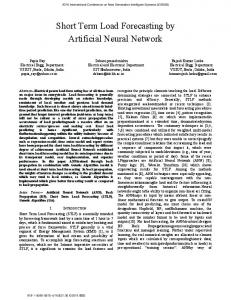
In this paper, we describe the implementation of an SOM to generate the load profile for the design of microgrids in terms of unit sizes. Most of the research in the literature on the generation of electricity demand profiles is based on real-time measurements. In this proposal, we include only socioeconomic aspects and some variables related to the consumption behavior of the community. The electricity forecast demand has been studied; however, there are few existing developments applied to microgrids which explicitly consider the characteristics of the demand, characteristics which are very different from those in traditional power systems. Also, in this paper, we propose for the operation of the microgrids an on-line neural network for load predictions, currently used as a key module in the energy management system (EMS) of a real microgrid system implemented in the north of Chile. Then, to keep track of changes in the behavior of the consumption, the parameters of the neural network models are continuously adapted including also the on-line measurements. The paper is organized as follows: In Section II, the load profile generation method based on SOM is described. Section III details the applied load forecasting using a neural network with on-line learning. In Section IV, the results for the real microgrid project ESUSCON are shown and discussed. In Section V the conclusions and suggestions for further research are presented. II. LOAD PROFILE GENERATION BASED ON SOM A. Self-Organizing Map (SOM) This section describes the self organization maps (SOM) developed by Kohonen [12][13]. One of the main features of the Kohonen’s SOM is their capability to classify complex sets of patterns in an unsupervised way, by extracting some classification criteria from the data, which are expressed and used later in a non-explicit manner [8]. This classification is carried out by using the distribution of an input space VI , over an output space Vo (usually of a lower dimension), and preserving the topological properties of the patterns in the input space. The output space is defined by a set of neurons generally arranged over a plane or a line, in a rectangular or hexagonal shape, where a neighborhood function is defined as shown in Fig. 1. The self-organized network must extract the important features, patterns, regularities, correlations or categories in the input data, and incorporate them in its internal structure of connections and links. The neurons must self-organize themselves based on the external stimuli, i.e., according to the inputs. After the learning process, an input vector x (x , … . . , x ) will activate the neuron j of the output space if the weighting ω , … . . , ω has the lesser distance to the input vector w vector x. In this way, the vector w is considered to be the prototype of the input space region whose vectors activate the neuron j (the so called winning neuron). In this way, two vectors with similar inputs according to the relations defined in VI will activate the same neuron or two different but near neurons of the output space.
x2
x1
INPUT LAYER x3
xn
wnj
w3j
w2j
w1j
..........
OUTPUT LAYER Fig. 1 Scheme of a Kohonen Neural Network.
The architecture of the SOM is a neural network with two layers. The input layer consists of n neurons one for each input variable. The neurons in the output layer are spatially distributed along a two-dimensional grid. Each input neuron i is connected to each output neuron j through a weight wij. Thus, the output neurons have a weight vector Wj called codebook which is a reference vector as it is the prototype (average) vector of the category represented by the output neuron j. In the basic training algorithm of the SOM, first the weights of the network are initialized. Then, a new input vector x is considered. After the activated neuron, whose weights are closest (in the Euclidean distance sense) to the vector x is found, the weight vectors of the activated neuron and its neighboring neurons are modified using the following equation: (
1)
( )
( ) ,
where x is the input vector, ω is the weight vector of the neuron j, and hjv() is a neighboring function. Generally, the neighboring area is based on the dynamic learning rate l , which changes dynamically during the learning process according to the equation: ( )
1
where l is a learning rate, c is constants (usually equals to 0.2), t is the current iteration and nn the number of neurons of the network [14]. Finally, the size of the neighborhood and the learning rate are continuously changing (or updated). This process is performed consecutively considering new input vectors x until the training process is finished. To visualize the SOM is usually not an easy task, because the classification process can be performed in high dimension spaces. One of the most popular methods to visualize the proximity relations of the reference vectors in a SOM globally is through an unified distance matrix U [15].
3
B. A New Method for Load Profile Generation Based on SOM In this paper, a new method to generate load profiles of residential electricity demand in isolated communities is proposed (see Fig. 2). In these communities, the energy supply is not available for the full 24 hour day. The main feature of the method is its capability of generating the electricity demand profiles by considering only the information obtained in a socio-economic survey conducted in the community, and without considering any measurement of the electricity demand in the past. The method is divided into three main components (see Fig. 2). In the first module of inputs, the information of each house in the community is obtained through surveys and site visits, which take place at each house. The information of the surveys is used in the second module of classification, where a SOM of Kohonen extracts the following information: classes, the elements of each class, and the features that differentiate each class. In the third module of search, a heuristic method is implemented. The characteristics of each class permit executing the search and assigning a profile that characterizes each class and then the total demand profile is obtained by multiplying by the number of the elements of each class. Each module is explained in details below.
Fig. 2 Procedure for Load Profile Generation Based on SOM
Input Module. This consists of obtaining relevant information from the community through well-structured surveys. Two methods of collecting the information are used: one is through the analysis of magazines, documents, and statistical data from various sources such as population and housing censuses, websites, and review of reports in libraries or in publications of governmental organizations. The other method is by the interviews in the field with the representatives of the relevant institutions of the town and the community itself, [16]. The individual surveys carried out in each house of the community are focused on obtaining information such as: number of persons living in the house, ages and occupations, incomes, number and type of electrical appliances, and hours of use of each appliance. In this module it is also very important to perform data processing, elimination of erroneous data, estimation of the missing data, numerical assignment of
qualitative variables obtained normalization of the data.
from the
surveys,
and
Classifier module. The main objective in this module is to obtain a classification of the different kinds of houses in the community in an unsupervised way, considering some criteria known a priori such as the number of family members, occupation of each of them, income, number of electrical appliances, and so on. The module will also provide information on the number of families in each class using an automated classifier. The classification of the houses is obtained by a self-organization, by making the neighbor neurons react more strongly to similar input patterns. In our case, as a measure of similarity we have chosen the Euclidean distance. The SOM does not require labels for each class; however, in order to reduce the complexity in the visualization process, the data could be labeled with for example the names of the family members, so that the results are visually easier to understand. Search Profile Module. For the searching process, a heuristic selection technique was used. The classifier considers the characteristics of all the classes and then in order to classify an input, it searches for the class with very similar characteristics in the database. The database is where demand profiles that define the classes are stored. The proposed method is suitable for communities that do not have a 24-hour energy supply, and thus, first, a data-base from another community with a 24-hour energy supply is required. Then, a metering system is installed at some houses and by using a survey, the characteristics of each house is obtained assigning a type of house. Then, the profiles of each type of house are stored. Initially, the database includes a certain number of predefined profiles; however, the database is flexible in the sense that it is possible to consider more and diverse profiles. The groups included in the database are: elderly couple, elderly person alone, elderly person and adult, adult alone, adult couple, couple with a child, adult couple with a teenager, couple with two young children, adult couple with two teenagers, couples with more than three children, and a profile assigned to those that do not correspond with any of the mentioned groups. Community demand profile. Finally, the total residential demand is obtained by summing the product of the number of elements in each class by the profile assigned to the class: ( )
( )
where dr is the total residential demand, c is the class, p(c) is the profile assigned to the class and ne(c) is the number of elements in the class. Note that this generated load profile is vital for sizing the microgrid distributed generation units during the microgrid project design stage.
4
III. LOAD FORECASTING USIN NG A NEURAL NETWORK WITH ONLINE LLEARNING For the electricity demand prediction, w we used a neural network trained on-line. In the Fig. 3, the m main steps of the forecasting procedure are shown. First, the ddata acquisition is performed. Then, after a pre-processing of the data, the requirements for the predictions are defined, such as sampling time, prediction horizon, step prediction,, etc. Finally, a neuronal network is identified and the loaad forecasting is obtained [17]. Each step is described below.
Data acquisition Data Pre-processing Requirements for the predicttion Modeling based on neural netw works
Electricity demand predictio on Fig. 3 Method for the Load Forecasting in the Microgrid
Data acquisition. First, the available measuured variables are determined. In this work, on-line measuremeents of the electric demand are available. This data is used for tthe training of the neural network. Data Pre-processing. Once data has beeen acquired, preprocessing must be performed: scalingg, missing data estimation, data correction, normalization, etcc. Requirements for the prediction. The paraameters needed to define the model and its future use are determ mined, such as the prediction horizon, the steps of prediction,, and the sample time of measures. Based on the requirementss, and considering all these parameters, the predictor is developeed. Modeling based on neural networks. Neural network identification is comprised of the following stteps (see Fig 4). Initial variable selection. This consists of ddetecting the most relevant variables. Correlation analysis oof the candidate variables is done. Data Selection. Once the variables of the moodel are obtained, the data is divided into three groups: trraining, test, and validation. The percentages 60%, 30%, annd 10% are used respectively.
Fig 4 Neural Network Identification
Definition of the initial structure of the neural network. The structure of the neural network k includes: (1) number of neurons in the input layer, which corrresponds to the number of inputs of the models obtained in th he initial variable selection step (this number is modified laterr in an optimization-based procedure to obtain the optimal inpu uts). (2) Number of hidden layers. The number of neurons in the hidden layer (in the initial structure twice the numbeer of the input layer is considered). (3) The nonlinear actiivation function (tansig is used). (4) One neuron in the output layer l with linear activation (function purelin). Training. On-line backpropagation trraining is used. onal structure optimization Optimization of structure. The neuro consists of determining the optimal inputs i to obtain a predictor with minimal error, and to determin ne how many neurons are optimal in the hidden layer (keep ping the balance of good prediction and complexity of the model). A sensitivity analysis is used for the selection of the relev vant inputs. The derivative of the output with respect to each h input is considered, and using a good threshold, the mo ost important inputs are determined [17]. Prediction. The prediction model caan predict within a horizon of two days or 192 periods of fifteen n minutes. Validation. Mean Squared Error (MSE), Mean Absolute v of the MSE are Percentage Error (MAPE), and variance considered as the performance index x. 1
1
100
where P is real power, P is the estimated e power, N is the number of data points (one hour N=4; N 12 hours N=48; 24 hours N=96; 48 hours N=192).
5
IV. CASE STUDY The proposed methods are used for the loadd profile generator and forecasting in a microgrid located in a small isolated village in the Atacama Desert, in northeern Chile called Huatacondo (20° 55' 36.37" S 69° 3' 8.71"" W). Its electric network is isolated from the interconnectedd system and the energy is supplied only during 10 hours eacch day by a diesel generator. A renewable based microgrid thaat takes advantage of the location and the availability of distrributed renewable resources in the area provides a 24-hour servvice to the village. Since the village experienced problems withh the water supply system, an integrated management soluution should be considered, including water consumption ttogether with the energy needed. Additionally, a demand side option to compensate the generation fluctuations caused by the mmarizes the key renewable sources is considered. Fig. 3 sum components of this microgrid, including phottovoltaic panels, a wind turbine, a diesel generator (typically aan existing unit in isolated locations), a battery bank, a water suupply system and a demand side-management mechanism (lloads) [18]. This renewable energy based microgrid project presents a novel way for integrating a community, through a SCADA system. The Social SCADA is developed withh the aim that communities perform the microgrid managging, maintenance tasks, consumption and generation monitoring, and decisionmaking processes, among others [19].
Fig 6 Electrical Applicancces of Huatacondo
ut data has 14 attributes In the second module, the inpu (dimensions), so we will have 14 neurons n in the input layer, and in total 24 houses were surv veyed. To determine the prototype vectors an SOM is used, and a for the visualization, a two-dimensional matrix-U. The outtput layer has 25 neurons (in a grid of Nx=3 by Ny=3. In Tab ble 1 the parameters of the SOM are presented. Initialization Size of map Neighboring function Shape of the map Coarse adjustment Detailed adjustment
Linear n Nx=3, Ny=3. Dimension A Gaussian n function Hexagonall Allows to o modify the activated neuron, a value v of 3000 was used Allows to modify the neighboring and the acttivated neurons, a value of 1000 waas used
Table 1 Parameters of the SOM
Fig. 5 Renewable-based Microgrid Diaagram
The survey results are classifieed identifying 7 types of families, as shown in Fig. 7. Th he hexagonal mesh with different colors represents the disstance. The groups were verified through a manual classiffication due to the small number of inhabitants. Figure 7 allows checking and verifying the coherence in the classification prrocess.
A. Results for the Load Profile Generaation Based on an SOM As explained in Section II, the proposal consists of three stages as detailed below. First, is the input module obtained from the surveys in situ. There are 31 houses, the number of inhabitants is 72, and there is one school inn the village. The individual survey provides the following infoormation: number of family members, age and occupation oof each member, family earnings, and domestic electrical appliiances. In the Fig. 6, the number of domestic electrical apppliances in the community of Huatacondo is shown.
Fig. 7 Classification of Huata acondo House Types.
6
The classification provides a class numbeer, characteristics of each class, and number of elements belongging to each class. That information is very important in the search stage, where the profiles are assigned according to the claass to which they belong. The third stage corresponds to the seaarch module that assigns a profile to each identified class in Huatacondo. The construction of the data base for Huatacondoo is the following: two assigned profiles corresponding to tw wo classes were obtained using real data of two types of housses from the rural community, Santa Rosa, Ecuador where there is 24-hour energy supply. The resting profiles were reeconstructed from these real profiles, and by using the surveyy information that projects the future for the use of the doomestic electrical appliances. Figure 8 shows the assigned profiiles of each class.
B. Results of Load Forecasting on n-line Learning based on Neural Network nal model is the electricity The available data for the neuron demand in the period from 02/12/2 2010 to 07/05/2011. This information is used for the neural network identification as t structural optimization presented in Section III, including the of the network. The identification n data was divided into: training, test, and validation. The predictions of the demand in the micro-network are used as input in the Energy Manageement System (EMS), in a rolling horizon procedure, with a sampling time of the optimizer of 15 minutes, and a contrrol horizon of 2 days [18]. The sampling time of the measurements is 15 minutes, and there are 192 prediction steps, equiivalent to the two days of prediction. he neural networks, we use For determining the structure of th a correlation analysis between th he electricity demand of Huatacondo and solar power, speed of wind, temperature, moisture, and solar radiation, from December, 2010 to July, 2011. The results are shown in Fig. 10. These variables do not have a higher correlation coefficientt; therefore the model uses only the historical demand. Thus, the inputs for the neural vious day with a sampling network are the demand of the prev time of 15 minutes (96 inputs). The Table 2 shows the characteristics of the neural network used, after the optimization stage.
Fig. 8 Electricity Demand Profiles of each Typee of Family in the Community of Huatacondo.
The profiles are multiplied by the numbber of families in each class, and then, the sum of the resullts represents the residential total demand in the Huatacondo coommunity. Figure 9 shows the load profile generated with the S SOM and the real Huatacondo load profile with uninterrupted supply, when the ESUSCON project was launched. In this figgure, the errors of each class and the high stochasticity featuress of the microgrid have an effect on the prediction of the tootal consumption; however, the trends are very similar andd useful as they generate a daily electricity demand profile of a community without measures of the consumption off electricity. The profiles were successfully used as a referencce in the planning stage, as the signal obtained was similar to tthe real electricity demand. This demand profile could be used to design electrification projects in communities, including the renewable resources.
Fig 10 Correlation of Electrical Demand and other Variables.
Neural Network Structure Number of layers Number of hidden layers Neurons of the input layer Neurons of the hidden layer Neurons of the output layer Activation function of hidden layeer Activation function of output layeer Training online Kind of training
3 1 96 8 1 Tansig Purelin Backpropagation Supervised
Table 2 Neural Network Structuree Used for Short-term Load Forecasting in Huatacondo
Fig. 9 Residential Daily Load Profile Generated d by SOM Method versus Huatacondo Actual Load Proofile.
Table 3 shows the average forecaast results of 20 days. The MAPE, MSE errors, and the vaariance are evaluated for different intervals: 1 hour, 12 hours, 1 day, and 2 days. The errors are increased when a longerr step-ahead prediction is
7
considered. The errors obtained are not com mpared with other methods because most of the latter are applied in traditional power systems. Electricity demand is more stochastic in the microgrids than in the traditional power syystems. Figure 11 shows the forecast for 2 days, MAPE 10%,, MSE 1.382 kW and variance 1.2 kW. Note that when more data is included, the MAPE and MSE index errors decrease. The real electricity demand is a stochasstic signal that is followed by the forecast electricity demand. The signals have low power, which is a feature of this small--sized micro-grid, and the main difficulty in the prediction iss that the energy demand of each house plays an important rolle in the total load profile. This is different from high scale ppower systems, in mal impact on the which the demand of each house has minim total demand profile. Time 4 1 hour
MAPE [%] 12.851
E MSE [kW W] 1..811
VAR [ kW] 1.379
48 12 hours
13.712
2..100
1.891
96 1 day
13.810
2..153
2.029
192 2 days
14.495
2..469
2.322
Stepahead
Table 3 Forecast Errors
Fig 11 Forecasting of Electricity Demand versu us Real Demand at Huatacondo
V. CONCLUSIONS In this paper, computational intelligence techniques are used to solve real-life problems in the Eneergy Management Systems of microgrids in small and isolatted communities. Kohonen self-organizing maps were implem mented to generate demand profiles, used for classifying electtricity demand of users; and neural networks perceptron m multi-layers were implemented to forecast electricity demand inn the microgrid. A method based on an SOM for generrating daily load profiles in isolated communities is presentedd. The community families are classified according to various aaspects and then a load profile is assigned to each class byy using an SOM classifier. This load profile generator can be uused to design the unit size of the distributed generators of m microgrid projects. The proposed load profile generator was tested using real data from the village called Huatacondo, obtaaining a demand profile quite similar to the real one. It must be noted that the demand in the valley and the peak zones occcurred during the
same hours of the real demand profille. Also, in this paper, a neural nettwork model with on-line learning for two days of load foreecasting is presented. The model considers a two-day step-aahead prediction horizon updated every 15 minutes with on n-line real measurements. This forecasting model is implemen nted as input for an Energy Management System of an isolated d real microgrid located at Huatacondo. ACKNOWLEDG GMENTS This work has been partially supported s by the mining company Doña Inés de Collahuasi,, the Millennium Institute “Complex Engineering System ms (ICM: P-05-004-F, CONICYT: FBO16, and FONDECY YT project 1110047.
References R NETWORK FOR SHORT – [1] F. Y. Xu, M. Leung, and L. Zhou, “A RBF TERM LOAD FORECAST ON MICR ROGRID,” in Machine Learning and Cybernetics (ICMLC), 2010 Internaational Conference on, 2010, vol. 6, no. July, pp. 3195–3199. [2] P. P. K. Chan, W. C. Chen, W. W. Y. Ng, and D. S. Yeung, “Multiple classifier system for short term load forrecast of Microgrid,” in Machine Learning and Cybernetics (ICMLC), 20 011 International Conference on, 2011, vol. 3, pp. 1268–1273. [3] Z. Bashir and M. El-Hawary, “Applyiing wavelets to short-term load forecasting using PSO-based neural neetworks,” Power Systems, IEEE Transactions on, vol. 24, no. 1, pp. 20–2 27, 2009. [4] V. H. Hinojosa and a. Hoese, “Shortt-Term Load Forecasting Using Fuzzy Inductive Reasoning and Ev volutionary Algorithms,” IEEE Transactions on Power Systems, vol. 25, no. 1, pp. 565-574, Feb. 2010. [5] N. Amjady and F. Keynia, “Short-term load forecast of microgrids by a new bilevel prediction strategy,” Smarrt Grid, IEEE, vol. 1, no. 3, pp. 286-294, 2010. [6] Y.-I. Kim, J.-M. Ko, and S.-H. Choi, “Methods for generating TLPs (typical load profiles) for smart grid--based energy programs,” 2011 IEEE Symposium on Computational In ntelligence Applications In Smart Grid (CIASG), pp. 1-6, Apr. 2011. [7] H. Mori and T. Itagaki, “A precondition n technique with reconstruction of data similarity based classification for short-term load forecasting,” in Power Engineering Society General Meeeting, 2004. IEEE, 2004, vol. 1, pp. 280–285. [8] S. Valero, J. Aparicio, C. Senabre, M. Ortiz, J. Sancho, and A. Gabaldon, “Comparative analysis of sellf organizing maps vs. multilayer perceptron neural networks for short-term load forecasting,” in Modern Electric Power Systems (MEPS), 2010 Proceedings of the International Symposium, 2010, no. 1, pp. 1–5. [9] S. Valero, J. Aparicio, C. Senabre, M. Ortiz, J. Sancho, and A. Gabaldon, “Analysis of different testin ng parameters in Self-Organizing Maps for short-term load demand forrecasting in Spain,” in Modern Electric Power Systems (MEPS), 2010 Proceedings of the International Symposium, 2010, no. 1, pp. 1–6. o Sarrion, A. Q. López, and I. N. [10] I. B. Sánchez, I. D. Espinós, L. Moreno Burgos, “Clients segmentation accord ding to their domestic energy consumption by the use of self-organiizing maps,” in Energy Market, 2009. EEM 2009. 6th International Con nference on the European, 2009, pp. 1–6. bre, A. G. Mar’\in, and F. J. G. [11] S. V. Verdú, M. O. Garcia, C. Senab Franco, “Classification, filtering, an nd identification of electrical customer load patterns through the use of self-organizing maps,” Power Systems, IEEE Transactions on, vol. 21,, no. 4, pp. 1672–1682, 2006. [12] T. Kohonen, “The self-organizing map,” Proceedings of the IEEE, vol. 78, no. 9, pp. 1464–1480, 1990. [13] T. Kohonen et al., “Self organization of a massive document collection.,” IEEE transactions on neural networks / a publication of the IEEE Neural 74-85, Jan. 2000. Networks Council, vol. 11, no. 3, pp. 57
8 [14] J. Kangas and T. Kohonen, “Developments and applications of the selforganizing map and related algorithms,” Mathematics and Computers in Simulation, vol. 41, no. 1, pp. 3–12, 1996. [15] J. C. Patra, E. L. Ang, P. K. Meher, and Q. Zhen, “A new SOM-based visualization technique for dna microarray data,” in Neural Networks, 2006. IJCNN’06. International Joint Conference on, 2006, pp. 4429– 4434. [16] C. Alvial-Palavicino, N. Garrido-Echeverría, G. Jiménez-Estévez, L. Reyes, and R. Palma-Behnke, “A methodology for community engagement in the introduction of renewable based smart microgrid,” Energy for Sustainable Development, vol. 15, no. 3, pp. 314-323, Sep. 2011. [17] D. Saez, M. Sanz-Bobi, and A. Cipriano, “Prediction of water chemical properties in the cycle of a coal power plant using artificial neural networks,” in Neural Networks Proceedings, 1998. IEEE World Congress on Computational Intelligence. The 1998 IEEE International Joint Conference on, 1998, vol. 3, pp. 1981–1986. [18] R. Palma-Behnke, C. Benavides, E. Aranda, J. Llanos, and D. Saez, “Energy management system for a renewable based microgrid with a demand side management mechanism,” in Computational Intelligence Applications In Smart Grid (CIASG), 2011 IEEE Symposium on, 2011, pp. 1–8. [19] R. Palma-Behnke, D. Ortiz, L. Reyes, G. Jimenez-Estevez, and N. Garrido, “A Social SCADA Approach for a Renewable based Microgrid – The Huatacondo Project –,” in Power and Energy Society General Meeting, 2011 IEEE, 2011, pp. 1–7.