Tripwire. H. 1.2. 7. 5. Auditd. H. 3.36. 9. 8. Snort. S,B. 6.72. 8. 3. Honeyd. S,B. 3.5. 8. 5. Nepenthes. S,B. 1.54. 8. 5. OSSEC. H. 4.32. 10. 3. IPFirewall (IPFW). S,B.
A Deployment Value Model for Intrusion Detection Sensors Siraj A. Shaikh1 , Howard Chivers1 , Philip Nobles1 , John A. Clark2 , and Hao Chen2 1
Department of Informatics and Sensors, Cranfield University, Shrivenham, UK {s.shaikh,h.chivers,p.nobles}@cranfield.ac.uk 2 Department of Computer Science, York University, York, UK {jac,chenhao}@cs.york.ac.uk Abstract. The value of an intrusion detection sensor is often associated with its data collection and analysis features. Experience tells us such sensors fall under a range of different types and are diverse in their operational characteristics. There is a need to examine some of these characteristics to appreciate the value they add to intrusion detection deployments. This paper presents a model to determine the value derived from deploying sensors, which serves to be useful to analyse and compare intrusion detection deployments.
1
Introduction
The value of an intrusion detection sensor is often associated with its data collection and analysis features. This is inevitable since so many of the sensors are designed with such characteristics in mind. Experience tells us such sensors fall under a range of different types and are diverse in their operational characteristics, some of which have been little studied. They offer a range of analytical abilities, with varying levels of efficiency, and incur a variety of costs. Hence, there is a need to examine these characteristics to appreciate the real value they add to sensor deployments. We present a model to help determine the benefit derived from deploying intrusion detection sensors at various locations in a network. The aim is to deploy sensors at locations in a systematic fashion such that maximum cumulative benefit is derived at a minimum cost. This builds on a broad characterisation of sensors identified in earlier work [1,2] which looks at sensor interaction abilities, locations in a network where such sensors could be placed, and costs involved in deploying and monitoring. Network locations are also characterised in terms of monitoring load incurred due to the amount of activity processed and cost of disruption due to extra installation required. The paper is organised as follows. Section 2 presents a characterisation of networks. Section 3 presents a characterisation of sensors. Section 4 presents the main contribution of this paper: a deployment value model to determine the benefit derived from placing a sensor at a location and a strategy to optimise the deployment of multiple sensors. Section 5 illustrates this using a case study. Section 6 discusses some related work and section 7 concludes the paper. J.H. Park et al. (Eds.): ISA 2009, LNCS 5576, pp. 250–259, 2009. c Springer-Verlag Berlin Heidelberg 2009 �
A Deployment Value Model for Intrusion Detection Sensors
2
251
Characterising the Network
We present network characteristics that help us to characterise the various deployment locations available in a network. Such locations are distinguished according to a variety of factors which affect sensor deployment. 2.1
Location Type
We specify three types of locations for sensor deployment: hosts (H), segments (S) and backbone (B) links. Each type provides different opportunities for placing a sensor and collecting some unique data: - Backbone links are the most commonly used location for this purpose where network traffic between hosts and parts of the network is monitored. - Segments allow such traffic to be monitored but are more useful for monitoring traffic within the same segment and link layer activity. - Hosts refer to clients or servers where process and application data is monitored. This is useful for detecting malicious code, including worms and viruses, system files, memory and processor utilisation, and logs. We use the three types of locations to classify sensors accordingly. LT and AT denote type for location L and sensor A respectively, and range over a given set of locations, LT , AT : {H, S, B}. Sensor A can be deployed over location L only if AT = LT . This ensures that sensors are deployed on compatible locations. 2.2
Load Factor
We specify load factor to denote the amount of processing due to monitoring involved at a location. For network links this corresponds to capacity and usage. Hosts are characterised by processing load in terms of processor and memory usage. Network locations where a high load factor is typical include - backbone links due to the amount of traffic that passes through, - network and application servers given the amount of processing involved both in offering services to a number of clients, and processing of data, - segments attached to busy servers or a large number of clients, and - gateways that serve to link the network to the outside world. We express load factor LF for a location L as LF (L) and restrict it to a range of values [1,10] to express relative load for different locations in a network. 2.3
Risk Profile
Chivers [3] introduces risk profiles for system components to characterise the risks to which a system is exposed to if the component is compromised. The notion could be applied to network nodes to denote the level of risk exposure for the network if particular nodes are compromised. This takes into account
252
S.A. Shaikh et al.
the value of a node as an asset, its location and the type of access it provides to penetrate further in a network, and the likelihood of intrusions targeting it. Risk profiles serve to highlight, for example, that web servers, critical to the operation of an organisation engaged in electronic commerce and likely to have more access to critical information, are at a higher risk than ordinary clients. We extend the notion to apply to segment and backbone links. A link provides an opportunity to detect compromise and a risk profile for a link is essentially a representation of the significance of such an opportunity. Calculation of risk profile also takes into account any preventative measures deployed to reduce risk exposure in parts of the network; the calculation includes - the aggregate risk profile of nodes attached, - the aggregate risk profile of other links attached, and - the risk reductive effect of any preventative measures deployed on the link. A risk profile for a location L is denoted as R(L) and expressed as a ratio relative to other locations within a network; the higher the R(L) the better the value of deploying a sensor at L. We restrict R(L) to a specific range [0,10]. 2.4
Disruption Cost
We identify disruption cost for locations to estimate the cost of deploying sensors. There are two factors to consider here. First, the cost of disruption at the location due to installation. This includes changes to configuration that may be necessary as a result of additional software or hardware deployed. Secondly, the critical importance of the location to the overall operation of the network. This represents the cost of disruption to the normal operation during installation. Such a cost is likely to manifest itself in terms of downtime, and a loss of services as a result. We denote disruption cost as D(L) for a location L and restrict it to a specific range [1,10], with a minimum such cost of 1.
3
Sensor Characteristics
We specify interaction abilities and efficiency, both of which are crucial to the capability of a sensor. Costs are also critical to assess the efficiency of a sensor. 3.1
Interaction Abilities
Individual sensors are represented in terms of their interaction abilities. This is the ability to understand and interact with protocol characteristics at various layers of the network. It may be limited to a single layer or span multiple service layers where at each layer a sensor may interact - to perform analysis using a range of data analysis techniques, - if need be, generate response to detect suspicious events, and - if possible, provide defense against such events. We use a range of values [1,10] to denote interaction AI for a sensor A. For each of the four service layers (Physical, Network, Transport and Application) it is assigned out of 2.50; AI is the cumulative total of values for each layer.
A Deployment Value Model for Intrusion Detection Sensors
3.2
253
Efficiency
Whereas interaction abilities are important to detecting various types of attacks, equally important is the performance of sensors to accurately detect events of interest. This could be expressed in terms of the likelihood of false positives and negatives. So, for example, a higher rate of false positives lowers the efficiency. We denote sensor efficiency AE for a sensor A as a fraction and restrict it to a particular range [0.1,1]. Since it serves to influence the interaction ability of a sensor, we use it to introduce a capability metric. Such a metric represents the effective monitoring capability of a sensor denoted as Cap(A) = AI × AE . 3.3
Costs
We take into account two different costs, deployment costs and monitoring costs. Deployment cost is a sum of both the cost CDep (A) of installing, configuring and maintaining a sensor A, and the cost D(L) of disruption at a location L. Network based sensors generally require minimal changes to network configuration; sensors placed inline require some rearrangements and may therefore be costlier. Host-based sensors are likely to be most costly to deploy given the disruption. Cost of deploying A over L is denoted CostD (A,L) = CDep (A) + D(L), where CDep (A) is restricted to a specific range [1,10]. Monitoring costs are to do with the use of a sensor to detect potentially suspicious events. For a given sensor A such costs include the human cost CMon (A) of manual engagement required for monitoring, and the load factor LF (L) for a location L monitored. Manual judgements required differs from sensor to sensor. Such effort is dependent on the load factor: the busier the location, the higher the levels of activity monitored, and therefore bigger the effort. The cost of monitoring using A at L is denoted CostM (A,L) = CMon (A) × LF (L), where CMon (A) is restricted to a specific range [1,10].
4
Deployment Value Model
We present a deployment value model for deploying a sensor in a network and present a strategy to optimally deploy a number of such sensors. 4.1
Deployment Value
Our characterisation of sensors and networks allows us to determine the value of sensors operating at particular locations in a network. The higher the capability deployed to mitigate the maximum risk, the higher the value of a deployment. For a sensor A and location L, assuming AT = LT , we denote deployment value V (A,L) for placing A over L as V (A, L) = (Cap(A) × R(L))/CostT (A, L) where CostT (A,L) denotes the total cost as a sum of deployment costs and monitoring costs for such a deployment CostT (A, L) = CostD (A, L) + CostM (A, L). Such a deployment is considered effective if V (A,L) ≥ 1, else it is deemed not to
254
S.A. Shaikh et al.
justify the costs involved. Note that the maximal value (120) for the total cost CostT (A,L) outweighs the maximal possible (100) for Cap(A) × R(L). This is acceptable since either the capability or the risk profile for a deployment should justify deployment costs at a minimum. 4.2
Deployment Strategy
We propose a deployment strategy to maximise deployment value of a set of sensors. We define a set of n sensors as SEN SORS = {ai | 0 ≤ i ≤ n} and a set of m locations as LOCAT ION S = {lj | 0 ≤ j ≤ m}. For some a ∈ SEN SORS and l ∈ LOCAT ION S we represent each placement, where a is placed at l, as a couple < a, l >. Given n sensors and m locations, a deployment is a set DEP of all such placements where the total number is equal to the lower of n and m. The challenge here is to determine the deployment value of a composition of sensors such that they are placed optimally, which, assuming all sensors are compatible with the location deployed at, ensures that placement is prioritised in terms of the maximum deployment value possible, while avoiding duplication of sensor capabilities at a location. Formally, DEP = {< ai , lj > | ∀ i, j • aiT = ljT ∧ai ∈ / {a1 , ..., ai−1 }∧lj ∈ / {l1 , ..., lj−1 }∧V (ai , lj ) ≤ V (ai−1 , lj−1 )} The construction of DEP ensures that for every placement -
location types of ai and lj are compatible aiT = ljT , sensor ai has not been deployed in a prior placement ai ∈ / {a1 , ..., ai−1 }, / {l1 , ..., lj−1 }, and location lj does not appear in a prior placement, lj ∈ deployment value of placing ai over lj is less than the deployment value of the previous placement V (ai , lj ) ≤ V (ai−1 , lj−1 )}.
The set DEP results in a list of compatible sensor-location pairings, all of which are unique and in descending order of deployment value. We check whether each individual deployment is of value 1 or more. A deployment value less than 1 represents an ineffective deployment where costs exceed the benefit. To factor it in we calculate the loss of benefit for each such deployment and offset it from the total deployment value. The deployment value operator is overloaded to extend over sets as V (DEP ) and represents the cumulative total value of all individual sensor placements such that if V (a, l) ≥ 1 then V (DEP ) = V (DEP ) + V (a, l), or if V (a, l) < 1, then V (DEP ) = V (DEP ) − (1 − (V (a, l)).
5
Case Study
We present an example network to demonstrate our model. Three different sensor deployment scenarios are chosen to reflect various host and network based sensors available. A list of sensors in Table 1 serves as a good variety some of which we use. It draws upon a characterisation of sensors from our earlier work [1,2], assigning capability and costs based upon use and experience.
A Deployment Value Model for Intrusion Detection Sensors
255
Table 1. A list of intrusion detection sensors Sensor (A) Type (AT ) Cap(A) CDep (A) CM on (A) Cisco IOS Port Security S 1.92 5 5 HP Virus Throttling H 6.39 8 2 Tripwire H 1.2 7 5 Auditd H 3.36 9 8 Snort S,B 6.72 8 3 Honeyd S,B 3.5 8 5 Nepenthes S,B 1.54 8 5 OSSEC H 4.32 10 3 IPFirewall (IPFW) S,B 2.8 6 4 Arpwatch S 0.48 2 5 Wireshark(Ethereal) S,B 2.75 2 9
5.1
Example Network
The network shown in Figure 1 comprises of two servers, on segment S1 , and two clients, on segment S2 . The backbone link B2 connects the two segments and the link B1 serves as the connection to the outside world. The two servers are labelled F T P and W W W to reflect the services they offer. They are the most significant asset to the network operator providing profitable services and incurring an expensive downtime, and are more likely to be targeted by intruders.
Fig. 1. An example network
256
S.A. Shaikh et al. Table 2. Risk, load and disruption cost assignments Location L LT R(L) LF (L) D(L) C1 H 1 1 1 C2 H 1 1 1 FTP H 5 7 8 WWW H 5 7 8 S1 S 4 7 6 S2 S 2 4 3 B1 B 9 9 9 B2 B 7 6 7
As shown in Table 2, we assign a risk profile of 5 to both servers and a 1 to both clients. The servers incur a disruption cost of 8 compared to the 1 for clients. The relative load factor for servers is also high, assigned a 7 to a 1 for clients. We assign a risk profile of 9 to B1 relatively higher to a 7 for B2 considering that B1 is exposed to externally sourced traffic which can potentially target servers or clients. Risk profiles 4 and 2 assigned to the two segments S1 and S2 respectively are due to the value of the hosts residing on them. The disruption costs 9 and 7 for B1 and B2 respectively reflect the level of disruption likely, while the load factor for the two locations has a similar ratio of 9 and 6 respectively. 5.2
Deployment Scenarios
We consider three possible deployment scenarios. Scenario 1 focuses on hostbased IDS solutions. Open Source Host-based Intrusion Detection System (OSSEC) is an open source solution that provides host-based intrusion detection and prevention. A total of four OSSEC clients are chosen to deploy at the four locations as shown in Table 3. Total deployment value adds up to -2.28. Sensors placed on the two servers add almost double the deployment value than the sensors placed on clients; such value is justified given that the servers are at a higher risk than clients despite higher costs. Deployment value indicates high costs of deploying an entirely host-based solution. Table 3. Deployment for Scenario 1 L A R(L) Cap(A) CostT FTP OSSEC 5 4.32 39 WWW OSSEC 5 4.32 39 C1 OSSEC 1 4.32 14 C2 OSSEC 1 4.32 14
V (A, L) 0.55 [-0.45] 0.55 [-0.45] 0.31 [-0.69] 0.31 [-0.69]
Scenario 2 focuses on network-based solutions. As shown in Table 4, two Snort sensors are deployed on the two most significant locations along with a switch port security mechanism on one of the segments. The total deployment value
A Deployment Value Model for Intrusion Detection Sensors
257
Table 4. Deployment for Scenario 2 L A R(L) Cap(A) CostT V (A, L) B2 Snort 7 6.72 33 1.43 B1 Snort 9 6.72 44 1.37 S1 Cisco IOS Port Security 4 1.92 46 0.17 [-0.83] Table 5. Deployment for Scenario 3 L A R(L) Cap(A) CostT V (A, L) B2 Snort 7 6.72 33 1.43 FTP HP VT 5 6.39 30 1.07 WWW HP VT 5 6.39 30 1.07
adds up to 1.97. The two Snort sensors are deployed on backbone links B1 and B2 , and the port security mechanism is deployed at S1 given the higher risk profile. The deployment value is significantly better than the first scenario. The second scenario benefits from a high capability sensor such as Snort deployed on the two most critical locations providing both near maximum visibility of the network at B2 , and monitoring traffic to and from the external gateway at B1 . Scenario 3 combines both types of sensors. As shown in Table 5 the two hostbased sensors are deployed on the two servers and a single Snort sensor is placed on the most significant link serving all externally sourced (and bound) traffic. The total deployment value is 3.56. Both backbone links are critical for monitoring both all traffic headed to and from the servers, and traffic passing in and out through the external gateway. While B1 provides visibility of all external traffic to and from the servers, it does not suffice as it fails to cover traffic between the internal segments. B2 provides good coverage but fails to offer any view of external traffic in and out of the clients on S2 . The Snort sensor is deployed on B2 given the better value compared to B1 ; this is primarily due to the higher cost incurred for deploying on B1 even though the risk profile for such a location is higher. The deployment value for the third scenario is almost double the value for second scenario. The deployment is designed such that the efficient host-based sensors are chosen for the two most valuable assets (servers), along with a single network-based sensor. The choice of deploying Snort on B2 over B1 is indicative of the costs involved with respect to the risk profile.
6
Related Work
Related work can be broadly divided in two categories: cost-benefit analysis of sensors taking into account efficiency and costs with disregard for the network deployed on [4,5,6], and placement of sensors in a given network characterised using system vulnerabilities but ignoring characteristics of sensors [7,8,9]. Lee et al [5] present a cost-benefit model deployments to evaluate data mining approaches to classifying and responding to intrusions in network traffic
258
S.A. Shaikh et al.
streams. They use various costs including intrusion damage, the type of response launched, and time and computational resources required for processing, to present a decision model for executing response to intrusions, where the lower the total cost the better the value. Factors such as detection efficiency and severity of configuration are not explicitly modelled; they are likely to impact response costs which determine consequential costs. Noel and Jajodia [7] present an approach for optimal sensor placement. They use attack graphs to represent possible paths taken by potential intruders to attack a given asset. Such graphs are constructed in a topological fashion taking into account both vulnerable services and applications that allow intruders to exploit nodes and use them as launch pads for further penetration, and protective measures such as firewalls deployed to restrict connectivity between nodes. Deployments are devised to monitor all paths using least number of sensors. This is dealt with as a set cover problem and a greedy algorithm is used: each router node allows for monitoring of certain graph edges and the challenge is to find a minimum set of routers that cover all edges. A vulnerability-driven approach [7] to deploying sensors overlooks factors such as traffic load on nodes. As a result the deployment is optimised such that the more paths that go through a node the more likely it is chosen for placement. The focus is limited on network-based sensors and sensor efficiency or costs are not modelled. Sheyner et al [9] present another approach based on attack graphs. They model networks as finite state machines and construct attack graphs using a symbolic model checker representing attacks as simple state transitions. Attack graphs produced in this way allow a network model to be automatically checked for a particular safety property given a set of permissible attacks. Minimisation techniques are used to deduce what attacks go undetected, what attacks should be prevented for the safety property to be satisfied, and using probabilistic information what is the likelihood of detecting particular attacks. The model [9] does not characterise the network or sensors; deployment value then becomes merely a measure of the likelihood of events being detected and prevented. Rolando et al [8] introduce a formal logic-based approach to describe networks, and automatically analyse them to generate signatures for attack traffic and determine placement of sensors to detect such signatures. Their notation to model networks is simple yet expressive to specify network nodes and interconnecting links in relevant detail. While there are advantages to using a formal model, such an approach may not be scalable. The formal notation allows for a more coarse-grained specification but it is not clear whether the resulting sensor configurations are even likely to be feasible for real environments. Moreover, the notation does not allow for modelling any system-level location or sensor characteristics. The approach is demonstrated for a limited class of attacks for which the logical predicates are simple to express. More complicated attacks will not be as simple to express and likely to incur considerable computational resources.
A Deployment Value Model for Intrusion Detection Sensors
7
259
Discussion
The deployment value model and strategy presented in this paper have been implemented using simple exhaustive search. Early results are promising for large scale deployments. Means to reason and compare intrusion detection sensor deployments are important to judge the ability of such sensors to make a difference individually or in combination. Our aim is to represent the complex relationship between the sensor and network characteristics in as simple a model as possible. The approach presented here has characterised a variety of features of sensors, and along with risk profiling and load characterisation for networks, such characteristics provide a system-smart view of sensor deployments. Work is underway to analyse large real deployments that serve to reflect on these aspects of the model. The current deployment strategy, adopted in Section 4.2, is designed to place sensors with a goal to maximise deployment value. Alternative strategies could be designed to emphasise risk reduction by improving the design of the network.
Acknowledgment This work is a joint effort by Cranfield and York universities, and funded by Engineering and Physical Sciences Research Council (EPSRC) (EP/E028268/1).
References 1. Shaikh, S.A., Chivers, H., Nobles, P., Clark, J.A., Chen, H.: Characterising intrusion detection sensors. Network Security 2008 (9), 10–12 (2008) 2. Shaikh, S.A., Chivers, H., Nobles, P., Clark, J.A., Chen, H.: Characterising intrusion detection sensors, part 2. Network Security 2008 (10), 8–11 (2008) 3. Chivers, H.: Security Design Analysis. York Computer Science Technical Report YCS 2006/06, University of York, UK (2006) 4. Cavusoglu, H., Mishra, B., Raghunathan, S.: The value of intrusion detection systems in information technology security architecture. Information Systems Research 16(1), 28–46 (2005) 5. Lee, W., Fan, W., Miller, M., Stolfo, S.J., Zadok, E.: Toward cost-sensitive modeling for intrusion detection and response. Journal of Comp. Sec. 10(1-2), 5–22 (1993) 6. Stakhanova, N., Basu, S., Wong, J.: A cost-sensitive model for preemptive intrusion response systems. In: 21st International Conference on Advanced Information Networking and Applications (AINA 2007), pp. 428–435 (May 2007) 7. Noel, S., Jajodia, S.: Optimal ids sensor placement and alert prioritization using attack graphs. Journal of Network and Systems Management 16(3), 259–275 (2008) 8. Rolando, M., Rossi, M., Sanarico, N., Mandrioli, D.: A formal approach to sensor placement and configuration in a network intrusion detection system. In: Proceedings of the 2006 International Workshop on Software Engineering for Secure Systems, pp. 65–71. ACM Press, New York (2006) 9. Sheyner, O., Haines, J., Jha, S., Lippmann, R., Wing, J.M.: Automated generation and analysis of attack graphs. In: Proceedings of the 2002 IEEE Symposium on Security and Privacy, pp. 273–284 (May 2002)