MODELING PATIENT SERVICE CENTERS WITH SIMULATION AND SYSTEM DYNAMICS
Thomas R. Rohleder Haskayne School of Business The University of Calgary 2500 University Drive NW Calgary, Alberta T2N 1N4 CANADA tel: (403) 220-7159 fax: (403) 282-0095 e-mail:
[email protected]
Diane P. Bischak Haskayne School of Business The University of Calgary
Leland B. Baskin Calgary Laboratory Services Dept of Pathology and Laboratory Medicine The University of Calgary
September 2006
Modeling Patient Service Centers With Simulation and System Dynamics
ABSTRACT We report on the use of simulation modeling for redesigning phlebotomy and specimen collection centers (or patient service centers) at a medical diagnostic laboratory. Research was performed in an effort to improve patient service, in particular to reduce average waiting times as well as their variability. Discrete-event simulation modeling provided valuable input into new facility design decisions and showed the efficacy of pooling sources of variation, particularly patient demand and service times. Initial performance of the redesigned facilities was positive; however, dynamic feedback within the system of service centers eventually resulted in unanticipated performance problems. We show how a system dynamics model might have helped predict these implementation problems and suggest some ways to improve results.
Keywords: DYNAMICS
SIMULATION,
HEALTHCARE,
FACILITY
DESIGN,
SYSTEM
1.
Introduction We report on a modeling study of outpatient phlebotomy and specimen collection
centers (patient service centers, or PSCs). Initially, our research focused on the use of discrete-event simulation to assist in the process of developing a template design for new facilities. However, problems encountered during the implementation phase led us to undertake additional modeling and analysis using system dynamics. In this respect our experience differs from that described in many previous discrete-event simulation modeling studies. Below, we elaborate on the path taken and the lessons learned. Like many health service organizations, Calgary Laboratory Services (CLS) was faced with increasing demand for its services but had limited resources available to meet that demand. A discrete-event simulation modeling study was commissioned to help senior decision makers at CLS determine the design of a more effective and efficient set of facilities.
Previous researchers have found discrete-event simulation to be useful in
assisting facility and process decisions in healthcare. Ashton et al. [1] used simulation to help a walk-in center identify problems and consider alternatives for waiting-room space and triage processes. Stahl et al. [2] used simulation to analyze alternative anesthesiologist staffing configurations to improve efficiency for surgery. Stafford and Aggarwal [3] set up a discrete-event simulation model of a university outpatient clinic; the model was used to explore the effects of different staffing levels and aggregation of two or more of the service units within the clinic. In their survey article on simulation in healthcare clinics, Jun et al. [4] provide a specific section on the effective allocation of resources, including the number and size of healthcare units. However, they note that simulation modeling to improve the operation
-1-
of multifacility networks is a neglected area of research. Swisher et al. [5] develop a discrete-event visual simulation model of an outpatient clinic that is planned to be part of a network of clinics, as they are interested in the effect of new facilities on existing ones, but their work so far has been based on a single facility. Indeed, to the best of our knowledge, no study has looked at the design or redesign of PSCs or similar healthcare facilities that form a network of locations within a large geographic area. Within the CLS network, the new facility implementation based on the suggested redesign of PSCs from our simulation model showed that patient waiting times and employee satisfaction were improved for the first several months. However, after approximately 18 months the new facilities were reporting significant problems with overcrowding, long wait times, and staff dissatisfaction. In part, these implementation issues could have been predicted with some thoughtful a priori system dynamics modeling. The predictive performance results might have helped CLS improve its implementation at the new facilities or at least to be better prepared for the challenging circumstances it would encounter. With the benefit of this hindsight, in this paper we emphasize the need for modelers to view studies dynamically, rather than as static projects. In particular, we see the need for modelers to have a complete toolset that evolves as studies unfold and helps organizations through all phases of design, implementation, and post-implementation. The remaining sections of this paper are as follows: a description of Calgary Laboratory Services’ operations; a report of the process, methods, and results of the discrete-event simulation model; a discussion of the implementation issues and proposed system dynamics model; and the conclusions and implications for management practice.
-2-
2.
Calgary Laboratory Services Calgary Laboratory Services provides a variety of medical testing services to the
population of Calgary, Alberta, Canada and surrounding areas. Services include standard tests on blood and urine, electrocardiogram (EKG), and a variety of specialized tests. Currently, CLS provides test results to approximately 2,200 physicians, who request over 15 million tests annually for the patient base of more than one million people1. CLS is a publicly operated organization. It serves the Calgary Health Region (CHR), which provides the majority of healthcare services in the Calgary area. The CHR determines the payment for tests performed by CLS and establishes performance standards such as patient waiting times and test turnaround times. Currently, CLS operates 18 PSCs, 4 hospital laboratories with their outpatient PSCs, a mobile collection service, a specimen pickup service from physician offices, and a centralized testing laboratory. Physicians are supplied with standardized test requisition forms to give their patients so that they can go to any of the 18 PSCs for service. (Some physicians generate their own requisitions.) The PSCs are spread out around the city and surrounding communities and are staffed primarily by lab technicians (laboratory assistants, LAs) who draw blood, perform EKGs, and prepare samples to be delivered to the testing facility by couriers. Prior to the formation of CLS by the merger of several independent laboratories in 1996, there were approximately 140 PSCs. By the late 1990’s, a network of 25 PSCs was established using a variety of policies (acceptable travel time, population allocation per
1
Information about CLS can be obtained at http://www.calgarylabservices.com/AboutCLS/CompanyProfile/ (last accessed 9/30/2006)
-3-
site, etc.). At that time substantial variability existed in the size of the PSCs. Some had as few as two staff members, while others had as many as 13 full-time and part-time employees. Patient waiting-time performance at these PSCs was as variable as their sizes. The standard performance target for waiting was that 80% of patients should be seen within 20 minutes of arriving at a PSC (“80/20”). At the time the present research started in the year 2000, some of the 25 sites were meeting this target while others were unable to achieve it for substantial periods of their operating hours. Much like other facilities in the health care systems of the U.S. and Canada, CLS was seeing increasing demand for their services due to a growing and aging population and the development of new testing technologies. Management at CLS thought that a new configuration of their network of PSCs might improve patient waiting times without significant commitment of new resources. In particular, they thought that operating fewer and larger PSCs might be beneficial. Such a pooling of resources is a well-known operations management technique to improve system performance in the face of variable demand across facilities. For example, Pasin et al. [6] used simulation to demonstrate that pooling of equipment across community healthcare service centers would reduce unit costs while maintaining current service levels.
As the initial step in the research
described here, faculty from the University of Calgary were invited to help evaluate designs for new facilities.
-4-
3.
The Discrete-Event Simulation Model
Rationale and scope After meeting with CLS management two of us (Author 1 and Author 2) quickly determined that the characteristics of the redesign problem required a descriptive and flexible modeling tool such as discrete-event simulation. For example, the PSCs faced random, non-stationary demand with significant peaks during the day, as shown in Figure 1. Such a demand pattern would be difficult to account for in analytic models, but incorporating this arrival stream into a simulation model as a non-stationary Poisson process is relatively straightforward (see, for example, Law and Kelton [7]). An additional modeling complication was the multi-stage nature of the process at a PSC. After patients arrived, they provided the test requisition from their doctor for data input and then waited for both a lab technician for service and a room to complete the testing. Not all patients followed the same path through the process, with some patients requiring an EKG in addition to giving blood and/or urine samples. Given these aspects of the system as well as the scheduled changes in staffing levels for full-time and part-time staff over the course of the day, it became clear that simulation was necessary to provide an informative assessment of system performance.
[INSERT FIGURE 1 ABOUT HERE]
The scope of the research was established by settling on the following objectives:
-5-
Provide an analysis of the current PSC configuration, including rough estimates of total resources required to meet the 80/20 waiting time service target for all facilities. Develop a template design for new, larger PSCs with the intent that CLS would gradually close current facilities and open new facilities based on the template. Provide other suggestions for improvements related to the operations and resources of the PSCs. Two specific issues that were intentionally excluded from the scope were developing optimized staff schedules (in part because CLS operated in a unionized environment) and identifying specific locations for new sites. It was recognized that both of these issues could significantly impact the design of PSCs. However, due to their political nature and their longer-term and strategic orientation they were omitted from the study. Further, the intent was not to identify an optimal configuration because practical constraints would not permit this. For instance, a single “mega” facility might have minimized the resources required to meet the waiting-time targets. However, this was not an acceptable solution to CLS due to issues with patient and employee travel and other factors. We chose to focus on how much improvement would be obtainable by moving to fewer, larger PSCs with a good design, recognizing that the design would continue to evolve, as would the domain of acceptable options.
Data collection and analysis The modeling process began with meetings of staff members and site visits of the researchers to PSCs. CLS had excellent data on patient arrivals and the services required
-6-
by these patients. Data for the various activity processing times (e.g., drawing blood (phlebotomy), EKG, etc.) were more difficult to obtain since tracking of these was not built into CLS’s information systems. These data were hand timed by CLS supervisors, and for some activities supervisor and staff judgment were used to provide estimates. Where possible, input analysis was performed to transform the data into representative mathematical functions for the simulation model. Table 1 shows sample results for three hours of patient interarrival time data. Each hour had to be analyzed separately due to the non-stationary arrival rate (see Figure 1). Table 1 supports the use of the exponential distribution; however, it should be noted that the statistical fit tests are not in full agreement and so the process included some “art” along with the objective science provided by the statistics. This approach is further demonstrated for the choice of distributions for two of the service time inputs: phlebotomy and EKG. Table 2 shows the distribution and p-values for the statistical fit. Just as important, however, were graphical comparisons for several distribution choices that were “close” in a statistical sense.
[INSERT TABLE 1 ABOUT HERE]
[INSERT TABLE 2 ABOUT HERE]
Verification and validation Verification of the simulation model was embedded in the modeling process as suggested by Kleijnen [8]. For example, to ensure the non-stationary arrival rate was modeled properly, patient input counts were compared hourly to ensure they matched the
-7-
expected inputs like those in Figure 1. Further, the “trace” function of the model-building environment was used to verify proper logic of patient flow. Finally, animation was viewed for multiple complete days of the terminating simulation to detect errors. PSCs were grouped into three different sizes that were considered representative of the 25 facilities that provided services at that time. Small sized PSCs were considered to be those facilities with patient volumes of fewer than 100 patients per day on average, medium sized PSCs saw an average of 100 to 200 patients per day, and large PSCs had an average patient demand of more than 200 patients per day. Simulation models were built for each size of PSC. Because CLS was chiefly concerned with patient service, they tracked performance on several service-oriented measures, including the number of patients processed per day, average patient waiting time, and the percentage of patients with waiting times over 20 minutes. The 95% confidence intervals generated from the simulation models for the latter two of these measures are shown in Figures 2a and 2b along with the actual values from a typical week at a particular PSC of the given size. For the large and medium sized facilities, the simulation model generally predicted results that were in line with actual facility performance; for the smaller facility, the simulation model predicted better waiting-time performance than that reported at the actual PSC. These results suggest that the model did not capture certain inefficiencies at this smaller PSC. This discrepancy was discussed with CLS supervisors and was deemed sufficiently explainable to consider the model appropriately valid, as staff suggested several reasons for the better performance predicted by the smaller facility model, including absenteeism and the training of new technicians, both of which would have a more significant impact on a smaller facility with fewer staff. In addition, as data
-8-
had been collected at many PSCs to ensure sufficient sample sizes to build the simulation model, the small, medium and larger models were really representative of “typical” sites in the size ranges. Across all operating PSCs there were some in each of the size ranges that had performance comparable to that of the model. The model results for patients waiting over 20 minutes at large facilities were also analyzed because the model predicted somewhat poorer performance than what was actually observed. The hypothesized reason for this discrepancy was shift management arrangements by supervisors at those PSCs that were contrary to CLS usual practice. Technicians would be asked to alter their break times and shift completions when the site was congested. However, this increased the average waiting time in other periods.
[INSERT FIGURES 2A AND 2B ABOUT HERE]
In addition to comparing output performance measures in order to validate the model, we also demonstrated an animated version of the model to various PSC supervisors and staff. Figure 3 shows the simple animation that was developed using the Arena simulation package [9]. The animation focused on the patient flow through the facility – much of the detailed logic was omitted to improve clarity. CLS staff agreed that the model represented the general conditions at the PSCs, with daily activity peaks that were representative of actual experience. In particular, CLS staff compared the clock time with the length of the waiting line and agreed it was similar to what they experienced in the PSC. Overall, we believed the model was sufficiently valid for our purposes of comparing different PSC designs. Also, because our objective was to evaluate the
-9-
potential of larger sites, the significant discrepancies with the small PSCs were of lesser concern. As Kleijnen [8] points out, a model will never be perfect, but should be “good enough” to attain its goal.
[INSERT FIGURE 3 ABOUT HERE]
Scenario analysis Once there was general comfort that the models represented actual operations to an acceptable degree, we ran several scenarios to explore the performance of alternative PSC template designs. We explored the idea of moving to networks of twelve or six facilities to take advantage of pooling demand and reducing individual PSC variability. A three percent patient demand growth rate was assumed since this was the approximate growth rate over the previous five years. We also assumed that demand could be spread evenly across the new set of facilities. We recognized this would be impossible to achieve in practice, but new facilities could be modified from the template to meet the specific demand requirements of a city region due to disparities in family growth, age, affluence, and other demographic factors. If no changes were made to the facility network, the projected performance of the CLS system in 2005 based on our discrete-event simulation model was a mean waiting time of over 52 minutes, with nearly half of patient waits exceeding the 20 minute target. Table 3 shows the results of simulations with the six and twelve PSC networks and the suggested resource configurations for each template facility. The model predicted that by better balancing the demand across the set of PSCs and taking advantage of resource
- 10 -
pooling, substantial performance improvement could be achieved. While in theory the six PSC scenario should take better advantage of the pooling effect than the twelve PSC scenario, the discrete nature of room and terminal resources led to better performance with twelve PSCs on some dimensions. In each case, no additional PSC staff was required and fewer overall resources were needed. For example, the 12 PSC design reduced front terminals by five units and EKG monitors by more than 30 across all facilities.
[INSERT TABLE 3 ABOUT HERE]
Recommendations Along with CLS management, we concluded that it would be wise to move toward a target of 12 to 15 PSCs. We targeted this range as opposed to a fixed target of 12 in recognition that the patient population and employees may have concerns with elimination of certain sites due to transportation and political issues. Reaching this range of facilities would require time since the leases on current sites had various expiration dates. We noted that site selection would be a key factor for success, but since this was not part of the project scope we made only very broad recommendations. In addition, we suggested several immediate resource changes (e.g., increasing the number of terminals) for some current facilities to help improve short-term performance. CLS carried forward with these recommendations, and a correspondence with a senior executive approximately six months after the completion of the initial study indicated that they were pleased with the results of implementing both the short and long term
- 11 -
recommendations. Performance at the newer, larger PSCs was very good with lower waiting times and improved staff morale.
4.
Delayed Implementation Issues – A Role for System Dynamics While we recognized potential implementation problems with shifting to fewer,
larger PSCs, we were encouraged by the initial positive feedback. However, approximately 18 months into the transition, stresses in the system were showing. CLS reported significant problems in meeting the waiting time targets at some of the new facilities. To add further to the confusion, they reported that some of the older, smaller facilities were performing better than the new PSCs. To alleviate management concerns that the original discrete-event simulation model was not valid, it was rechecked with current data from a different PSC. The model was still accurate, but demand levels were significantly greater than originally predicted. For some sites, demand was more than 25% greater than original projections. Could this have been anticipated? To help answer this question we developed a system dynamics model of the opening of a new facility. System dynamics was identified by Young [10] as an appropriate method for improving healthcare management and was used in healthcare environments to explore policies for ongoing operations such as emergency departments [11-12]. Here, we describe a somewhat different use of system dynamics modeling. At the time of implementation of the new facility design there were no data on how the design would itself affect the network of PSCs. However, system dynamics can be used to forecast potential outcomes and as a qualitative learning tool. For example, Taylor and
- 12 -
Dangerfield [13] used two cases of a shift in the location of cardiac catheterization services to develop a system dynamics model to explore the potential effects of alternative policies on the demand for services. An advantage of system dynamics as pointed out by Sterman [14] is to help decision makers get out of the typical eventoriented view of the world where a problem (inconsistent PSC waiting-time performance) is identified and decisions (to move to fewer, larger facilities) are made to try to achieve particular results (shorter waiting times) in a linear fashion without considering potential feedback effects caused by the decision.
Developing the system dynamics model Many of the potential feedback effects and system time delays were known at the time of the original decision, although exact quantification of these factors would have been difficult. However, the behavioral consequences of opening new PSCs could have been explored and used to help understand implementation results or even to improve the implementation process. Figure 4 shows a system dynamics model that incorporates some of the key feedback mechanisms and time delays affecting PSC demand. The +s and –s in the diagram represent the polarity effects of the “cause” variable on the corresponding “effect” variable. As an example, as Waiting Time increases, Patient Satisfaction decreases (ceteris paribus). In the figure, the “Bs” and looping arrows represent balancing feedback loops in the system. For instance, the Word of Mouth loop increases PSC use when waiting times are low due to satisfied patients telling their friends and family. As waiting time increases, the rate of PSC use from Word of Mouth will decline.
- 13 -
[INSERT FIGURE 4 ABOUT HERE]
As reported by Kaldenberg and Becker [15], word of mouth is very influential when patients make healthcare choices. Further, the authors report that aspects of patient care that deal with access to service, such as length of waiting time, are typically given lower performance ratings by health care consumers than other service attributes and increasingly play a role in patients’ site selection. Since PSCs are relatively close together, it is not difficult for patients who hear that a new PSC has shorter waits to move to a different location from their nearest (or usual) site in an attempt to avoid waiting. The responsiveness of the system to word of mouth is affected by the Visit Lag Time parameter in the model. As opposed to customers visiting an overcrowded bank branch, most patients visit the PSCs relatively infrequently. To incorporate this effect in the system dynamics model, we assume an average time of 6 months between visits. Thus people will update their knowledge of performance at the PSC relatively slowly. Patients start using the new PSC as Incoming PSC Users, and the submodel presented in Figure 5 shows how the flow of patients to a new PSC begins. The longer the PSC is open (shown by the stock: PSC Age), the more prospective users of the PSC become actual users due to increased knowledge of the facility. The PSC Knowledge Factor mathematically represents this process with the function 1 - e-L/ , where L is the length of time the PSC has been open and
is a normalizing constant (1 month). This
factor starts at zero and approaches 1 (full knowledge) asymptotically as L increases. For modeling purposes, the number of Base PSC Users was set at 1000 (the initial value for Possible PSC Users) and the Capacity of the new facility was set at 100 patients per
- 14 -
month, although any values can be used to represent a particular facility. The system dynamics model was therefore structured to provide insight into the expected demand and performance dynamics for a new “generic” site as opposed to modeling any one site specifically. We further assumed a 3% growth rate for the Possible PSC Users due to population growth and an aging demographic. For Figures 4 and 5, the boxes represent stocks where the flows from the double lined arrows accumulate (or decline). The “valve” represents the rates of inflow and outflow. Also, with the growth rate, a reinforcing loop (designated with the “R” in the full explicit model in the Appendix) is created that drives PSC demand upward.
[INSERT FIGURE 5 ABOUT HERE]
Evaluating the system dynamics model and results The submodels of Figures 4 and 5 were combined and run for 60 months using the Vensim system dynamics modeling software [16]. Model building was performed in an iterative manner with client involvement as suggested by Lane et al. [17]. Additional testing of the model was also performed as prescribed by Sterman [18]. Table 4 shows some of the tests performed and examples of results. The model passed all of these tests, so we viewed it as valid for providing useful insights into system behavior. Therefore, we moved to running the model and exploring its outputs.
- 15 -
[INSERT TABLE 4 ABOUT HERE]
Figure 6 shows the resulting behavior of the model for three key variables. PSC Visits grow quickly during the first several months as patients discover the new PSC and because low wait times lead to high satisfaction. This causes patients to encourage family and friends to go to the new PSC (at the rate indicated by the Friends and Family Visitors path). However, due to the time lags inherent in the system, demand significantly overshoots the capacity of 100 – leading to excessive waiting times. Visitation to the new PSC does eventually go down, but again the rate of switching to another PSC (PSC Switchers) lags behind the peak demand period. With the base parameters selected it is interesting that the peak demand period coincides with the timing of PSC management’s return call to the research team (this includes about six months for the new larger PSC policy to be implemented).
[INSERT FIGURE 6 ABOUT HERE]
The model helps explain the oscillating demand dynamics of the opening of a new PSC and the overall effects of a positive growth rate. A priori it would be difficult to quantify the exact results, but sensitivity analysis showed that the general behavior of the model remained nearly identical within a reasonable range of parameter values (e.g., three to nine months for Visit Lag Time). Therefore, the insights could be useful for
- 16 -
handling the implementation process. At a minimum, knowing that demand could be substantially greater than desired could help prepare the facility for the onslaught. The model can also be used to explore policy options to help alleviate the demand peak. While there are not many management levers in this process, perhaps the key one is advertising the availability of a new PSC. By aggressively advertising the new facility, the PSC User Population would start at an initially larger level and perhaps mitigate the overshoot effect. Figure 7 compares the base case results with the model result when the new PSC is advertised and the initial PSC User Population starts at 50% of the total Possible User Population. The figure shows that if the majority of potential users are aware of the new facility the overshoot effect can be avoided, eliminating the resulting system imbalance.
[INSERT FIGURE 7 ABOUT HERE]
Due to the lag time in visitation already discussed, it would be very difficult to inform all patients of the new facility. However, obvious choices of those to inform to effectively control demand would be frequent users and institutional users such as nursing homes. Such patients’ immediate impact on the PSC waiting times would help control the potential overshoot in demand. While the intent of the system dynamics modeling was to demonstrate its potential use as a predictive tool and to improve insight into PSC system problems, Figure 8 shows PSC visitation data from an actual facility. This particular location was an enlargement of an existing site, so many users already knew of its existence (similar to
- 17 -
the case with advertising discussed above). Nonetheless, the pattern of visitation shows the overshoot and oscillating behavior similar to the dynamic model. The actual anecdotal evidence and these data seem to suggest a significant degree of model validity. Note also that since the original dynamic model was developed before these data were available, its availability did not bias model development.
[INSERT FIGURE 8 ABOUT HERE]
Conclusions In this paper we discussed the role of discrete-event simulation and system dynamics modeling for redesigning and implementing patient service centers. Results from the discrete-event simulation model suggested that the organization involved, Calgary Laboratory Services, should move to larger and fewer facilities for its PSC network to take advantage of the “pooling” effect to reduce demand variability and improve resource utilization. Scenarios were run that considered reducing the number of sites by 50-75%. The discrete-event simulation model predicted that this move would allow CLS to meet its patient service target that required 80% of patients to have waiting times less than 20 minutes, whereas the current configuration would substantially miss that target. CLS has moved in this direction, going from 25 facilities in 2000 to the current 18 PSCs. This evolution has not been without its implementation challenges due to unexpected levels of demand caused, in part, by internal system feedback. Determining the effects of the feedback would have been difficult without the aid of a model due to time lags and the complex behaviors of patients. We showed how system dynamics could
- 18 -
have helped to predict some of the patterns in demand and perhaps suggest policies to reduce demand variability over time. As an overall recommendation, we believe that when redesigned facilities or operations result from a detailed modeling exercise similar to the one described herein, system dynamics may be a useful tool for exploring the possible side effects of the new system. Even simply the creation of a causal loop diagram like that in Figure 4 may provide valuable insight. However, the development of a full dynamic model would be even better, since it may help in predicting and/or understanding unanticipated results. As healthcare systems and organizations like CLS continue to deal with challenges in meeting increasing demand with limited resources, they will undoubtedly be asked to make significant changes in how they operate. Modeling tools like discreteevent simulation can be very valuable in helping make good decisions to improve performance.
As suggested by Harper and Pitt [19], carefully managing healthcare
modeling projects such as this one is a key to success. We would further assert that modeling in health care really needs to be viewed as an ongoing process. Any change in the operations of the system will have side effects that over time can have significant impact on patient care and overall system performance. Additional tools like system dynamics can aid in understanding the effects of changes to these complex systems. As the changes progress, new data from the system can be used to further modify designs and smooth implementation. Going into a modeling effort with the view that it is a process rather than a discrete project will help all involved achieve the long-term results desired.
- 19 -
Appendix Explicit System Dynamics Model Conversation Delay
+ Patient Satisfaction -
Friends and Family + B Population Send Friends and Family + Word of Word of Mouth Mouth Factor
Incoming PSC Users
-
Aging Rate
+
PSC Knowledge Factor
Capacity
Waiting Time + PSC Visits +
+Visit Lag Time
+
Satisfaction Conversion Factor
B No Time to Wait
PSC User Population
Emigration Rate +
-
PSC Switchers R
Potential Returning Demand
+ Natural Emigration
System Growth (or Decline)
+ Choose New PSC + -
+ Possible PSC Users Incoming Possible Users +
PSC Age Tau Factor
Base Possible Users
Growth per Month
Equation and Parameter Values (with Units) Aging Rate ~ Rate that new PSC ages: 1 (Month/Month). Base Possible Users ~ Initial number of potential patients for new PSC: 1000 (Patients). Capacity ~ Capacity of PSC: 100 (Patients/Month). Choose New PSC ~ Rate that potential patients choose to go to new PSC: (Possible PSC Users*PSC Knowledge Factor)/Visit Lag Time (Patients/Month). Conversation Delay ~ Delay time for communication between patients: 6 (Month). Emigration Rate ~ Rate at which patients depart region: 0.01 (Dmnl2/Month). Friends and Family Population ~ Population of friends and family available to PSC users: Possible PSC Users*Word of Mouth Factor (Patients). Growth per Month ~ Growth rate of patients: 0.03 (Dmnl/Month). Incoming Possible Users ~ Rate at which new potential patients arrive: Growth per Month*Potential Returning Demand (Patients/Month). Incoming PSC Users ~ Rate of patients joining new PSC User Population: Choose New PSC+Send Friends and Family (Patients/Month).
2
Dmnl = Dimensionless
- 20 -
Natural Emigration ~ Rate of patients leaving the system: Emigration Rate*Potential Returning Demand (Patients/Month). Patient Satisfaction ~ Satisfaction level of patients based on waiting time: SMOOTH((Satisfaction Conversion Factor-Waiting Time)/Satisfaction Conversion Factor,Conversation Delay): (Dimensionless). Possible PSC Users ~ Population of potential patients: Incoming Possible Users-Choose New PSC (Patients). Potential Returning Demand ~ Based on overall system demand this stock is the potential return users: PSC Switchers-Natural Emigration (Patients). PSC Age ~ Age of new PSC: Aging Rate (Month). PSC Knowledge Factor ~ Factor representing possible user knowledge of new PSC: 1EXP(-PSC Age/Tau Factor) (Dimensionless). PSC Switchers ~ Rate at which dissatisfied patients stop using PSC: (PSC User Population*(1-Patient Satisfaction))/Visit Lag Time (Patients/Month). PSC User Population ~ Patients using the new PSC: Incoming PSC Users-PSC Switchers (Patients). PSC Visits ~ Patients visiting PSC each month: PSC User Population/Visit Lag Time (Patients/Month). Satisfaction Conversion Factor ~ This factor converts waiting time into patients satisfaction: 100 (Months/Patient). Send Friends and Family ~ Based on the rate of satisfaction, patients send friends and family to the new PSC: (Patient Satisfaction*Friends and Family Population)/Visit Lag Time (Patients/Month). Tau Factor ~ Normalizing constant: 1 (Month). Visit Lag Time ~ Time between patient visits to PSC: 6 (Months). Waiting Time ~ Based on patient demand and capacity, the estimated waiting time (bounded by a maximum of 100): IF THEN ELSE( Capacity > PSC Visits, Min((PSC Visits/Capacity)/(Capacity-PSC Visits)*100,100) , 100 ) (Month/Patients). Word of Mouth Factor ~ Effectiveness of satisfied patients’ conversion of friends and family: 0.25 (Dimensionless).
- 21 -
References [1]
R. Ashton, L. Hague, M. Brandreth, D. Worthington, and S. Cropper, A simulationbased study of a NHS walk-in centre, Journal of the Operational Research Society 56 (2005) 153-161.
[2]
J.E. Stahl, D. Rattner, R. Wiklund, J. Lester, M. Beinfeld and G. S. Gazelle, Reorganizing the system of care surrounding laparoscopic surgery: a costeffectiveness analysis using discrete-event simulation, Medical Decision Making 24 (2004) 461-471.
[3]
E. F. Stafford Jr. and S. C. Aggarwal, Managerial analysis and decision-making in outpatient health clinics, Journal of the Operational Research Society 30 (1979) 905-915.
[4]
J. Jun, S. Jacobson, and J. Swisher, Application of discrete-event simulation in health care clinics: a survey, Journal of the Operational Research Society 50 (1999) 109-123.
[5]
J. R. Swisher, S. H. Jacobson, J. B. Jun, and O. Balci, Modeling and analyzing a physician clinic environment using discrete-event (visual) simulation, Computers and Operations Research 28 (2001) 105-125.
[6]
F. Pasin, M. H. Jobin, and J. F. Cordeau, An application of simulation to analyse resource sharing organisations among health-care organisations, International Journal of Operations and Production Management 22 (2002) 381-393.
[7]
A.M. Law and W.D. Kelton, Simulation Modeling and Analysis, 3rd ed. (New York: McGraw-Hill, 2000).
- 22 -
[8]
J. Kleijnen, Verification and validation of simulation models, European Journal of Operational Research 82 (1995) 145-162.
[9]
Arena, Version 5.00 (Rockwell Automation 2000).
[10] T. Young, An agenda for healthcare and information simulation, Health Care Management Science 8 (2005) 189-196.
[11] S.C. Brailsford, V. A. Lattimer, P. Tarnaras and J.C. Turnbull, Emergency and ondemand health care: modelling a large complex system, Journal of the Operational Research Society 55 (2004) 34-42.
[12] D.C. Lane, C. Monefeldt, and J.V. Rosenhead, Looking in the wrong place for healthcare improvements: A system dynamics study of an accident and emergency department, Journal of the Operational Research Society 51 (2000) 518-531.
[13] K. Taylor and B. Dangerfield, Modelling the feedback effects of reconfiguring health services, Journal of the Operational Research Society 56 (2005) 659-675.
[14] J.D. Sterman, System dynamics modeling: tools for learning in a complex world, California Management Review 43 (4) (2001) 8-25.
[15] D. O. Kaldenberg, and B. W. Becker, Evaluations of care by ambulatory surgery patients, Health Care Management Review, 24 (3) (1999) 73-83.
[16] Vensim, Version 5.4 (Ventana Systems, Inc. 2003).
[17] D. C. Lane, C. Monefeldt, and E. Husemann, Client involvement in simulation model building: hints and insights from a case study in a London hospital, Health Care Management Science, 6 (2003) 105-116.
- 23 -
[18] J.D. Sterman, Business Dynamics: Systems Thinking and Modeling for a Complex World (Boston: Irwin McGraw-Hill, 2000).
[19] P.R. Harper and M.A. Pitt, On the challenge of healthcare modelling and a proposed project life cycle for successful implementation, Journal of the Operational Research Society 55 (2004) 657-661.
- 24 -
Figures
Arrivals
Typical Daily Demand Pattern at a PSC 50 40 30 20 10 0 6:30:00 AM
8:00:00 10:00:00 12:00:00 2:00:00 AM AM PM PM
4:00:00 PM
6:00:00 PM
Tim e of Day
Figure 1: Non-Stationary Demand at CLS
95% confidence intervals and actual average waiting time, for three PSCs (3=Large, 2=Medium, 1=Small)
PSC 3
PSC 2
PSC 1
0
5
10
15
20
25
30
35
40
45
50
Average w aiting tim e in m inutes
Figure 2a: 95% confidence intervals and actual average waiting time for three PSCs
95% confidence intervals and actual percentage of patients with greater than a 20 minute wait, for three PSCs
PSC 3 PSC 2
PSC 1
0
10
20
30
40
50
60
70
Percentage of w aits greater than 20 m inutes
Figure 2b: 95% confidence intervals and actual percentage of patients with greater than a 20 minute wait, for three PSCs
Figure 3: Animation of an Example PSC
Dynamic Model of Opening a New Patient Service Centre Patient Satisfaction + B Send Friends and Family Word of Mouth
+
Visit Lag Time
Incoming PSC Users
Capacity
Waiting Time
B
+ PSC Visits + PSC User Population
No Time to Wait + PSC Switchers -
Figure 4: Causal Loop Diagram of PSC User Population
Flow of Patients to a New PSC
Incoming PSC Users
+
PSC Knowledge Factor
+ + Choose New PSC +
Aging Rate
PSC User Population
Possible PSC Users Incoming Possible Users + Growth per Month
PSC Age Base Possible Users
Figure 5: Patient Inflow Submodel
Dynamics of New PSC Visitation 150
100
50
0 0
6
12
18
24
30 Months
36
42
48
PSC Visits PSC Switchers Friends and Family Visitors Figure 6: Results of System Dynamics Model
54
60
Patients/Month Patients/Month Patients/Month
Effective Advertising vs. Base Case 150
100
50
0 0
6
12
18
PSC Visits with Advertising PSC Visits Base Case
24 30 36 Time (Month)
42
48
54
60
Patients/Month Patients/Month
Figure 7: Comparison of Advertising New PSC vs. Base Case
Actual PSC Demand Data 140
Scaled Demand
120 100 80 60 40 20 0 1
3
5
7
9
11
13
15
17
19
21
23
Month
Figure 8: PSC Visits for a New Facility - Actual Data Due to seasonalities in PSC demand, the scaled demand was adjusted based on several years of overall system demand.
Tables
Table 1. Patient Inter-Arrival Time Data Fit Analysis with Exponential Distribution p-value (reject distributional choice for small values, e.g. < 0.05) Time
Chi-squared
Anderson-Darling
Kolmogorov-Smirnov
8 – 9 a.m.
0.2710
≤ 0.05
> 0.25
9 – 10 a.m.
0.1562
0.025
0.10 ≤ p ≤ 0.15
10 – 11 a.m.
≤ 0.01
0.01 ≤ p ≤ 0.02
0.05 ≤ p ≤ 0.10
Table 2. Service Time Input Distribution Analysis Service
Sample Size
Distribution Choice
Chi-squared p-value
Phlebotomy
50
Gamma(2.01,1.5) + 0.85
0.0638
EKG
30
Loglogistic(-0.36,4.72,4.61)
0.2692
Table 3: Configurations and Results for New Template PSC Designs Resource/Performance
6 PSCs
12 PSCs
24 FTE’s *
12 FTE’s
Front Terminals
5
3
Phlebotomy Rooms
5
3
EKG Rooms
2
1
4.1 Minutes 4.7%
2.1 Minutes 1%
Staff
Performance Mean Waiting Time % > 20 Min. Wait (FTE = Full time equivalent)
Table 4: Examples of Assessment Tests of the System Dynamics Model Test
Example Result
Extreme Condition
Visit Lag Time = 0: PSC Visits go to infinity (expected result) Visit Lag Time = 100: PSC Visits drop to near zero (expected result)
Structural Assessment
If stock of Possible PSC Users drops to zero, there are zero users to Choose New PSC
Dimensional Consistency
Software automatic check = passed Equation inspection showed no anomalous dimensions
Integration Error Test
Shortening the time step by a factor of 10 has almost no effect on model results (test passed)