A Design Flow for Partially Reconfigurable Hardware - Semantic Scholar

A Design Flow for Partially Reconfigurable Hardware IAN ROBERTSON and JAMES IRVINE University of Strathclyde

This paper presents a top-down designer-driven design flow for creating hardware that exploits partial run-time reconfiguration. Computer-aided design (CAD) tools are presented, which complement conventional FPGA design environments to enable the specification, simulation (both functional and timing), synthesis, automatic placement and routing, partial configuration generation and control of partially reconfigurable designs. Collectively these tools constitute the dynamic circuit switching CAD framework. A partially reconfigurable Viterbi decoder design is presented to demonstrate the design flow and illustrate possible power consumption reductions and performance improvements through the exploitation of partial reconfiguration. Categories and Subject Descriptors: B.5.2 [Register-Transfer-Level Implementation]: Design Aids—automatic synthesis; B.6.3 [Logic Design]: Design Aids—simulation, verification, hardware description languages; C.5.4 [VLSI Systems]; E.4 [Coding and Information Theory]: Error Control Codes; I.6.m [Simulation and Modeling]: Miscellaneous; J.6 [Computer-Aided Engineering]: Computer Aided Design (CAD) General Terms: Design, Performance, Verification Additional Key Words and Phrases: FPGA, dynamically reconfigurable logic (DRL), run-time reconfiguration (RTR), Viterbi decoder, power estimation, configuration control

1. INTRODUCTION This paper presents a top-down, designer-driven design flow and the dynamic circuit switching (DCS) computer-aided design (CAD) framework for creating partially reconfigurable designs. The design flow begins with descriptions of the design’s hardware in VHDL and a reconfiguration information format (RIF) file, to describe its reconfigurable behavior. The design is partitioned into tasks, each of which is represented by a component. The top level of the design is therefore structural. Within each component, any level of abstraction can be used (behavioral, register transfer level (RTL), or structural). The dynamically reconfigurable logic (DRL) design process is more complex than conventional design. Therefore, it is vital to verify early on the correct capture of the designer’s intent, and the functional correctness of the overall design. If verification is This research was supported by the EPSRC, award number 99309356. Author’s address: Department Electronic and Electrical Engineering, University of Strathclyde, Royal College Building, 204 George St., Glasgow G1-1XW, UK; email: [email protected]. Permission to make digital/hard copy of part of this work for personal or classroom use is granted without fee provided that the copies are not made or distributed for profit or commercial advantage, the copyright notice, the title of the publication, and its date of appear, and notice is given that copying is by permission of the ACM, Inc. To copy otherwise, to republish, to post on servers, or to redistribute to lists requires prior specific permision and/or a fee. ° C 2004 ACM 1539-9087/04/0500-0257 $5.00 ACM Transactions on Embedded Computing Systems, Vol. 3, No. 2, May 2004, Pages 257–283.

258

•

I. Robertson and J. Irvine

only performed near the end of the design cycle, then the delay before bugs are found is unacceptably long. The DCSim tool can create a simulation model of the reconfigurable design capable of modeling the full design, its reconfigurations, including the reconfiguration interval, and automatically detecting many reconfiguration sequencing errors. Once the design is functionally correct, synthesis and automatic placement and routing (APR) tools are required to implement it. However, conventional implementation flows are designed for static designs and cannot be applied directly to dynamic designs. DCSTech can partition the dynamic design into a set of sub-designs for separate implementation by conventional CAD tools. This can be though of as dynamic-to-static conversion. After synthesis and APR, the design’s timing can be accurately estimated. Commercial APR tools typically provide gate-level design descriptions along with standard delay format (SDF) timing files. Using these files, DCSTech can build a gate-level timing model of the dynamic design. From this, DCSim can construct a timing simulation model to evaluate the design’s overall performance. Implementation of the design requires partial configuration files, but commercial CAD tools provide full configurations in most cases and DCSBitstream is used to extract partial configurations from these full configurations. A dynamic design requires a configuration controller to sequence and control reconfigurations. It can be implemented in a variety of ways, using hardware or software and can vary widely in complexity. Software allows the implementation of complex control algorithms like hardware operating systems [Brebner 1996], but often cannot match the performance of a dedicated hardware controller. DCSConfig can be used to automatically synthesize a hardware controller from information in the RIF file. Including this controller in DCSim’s simulations gives a more realistic picture of the design’s performance during reconfiguration. This paper begins by reviewing existing research into CAD tools and techniques for run-time reconfiguration (RTR) in Section 2, before describing the operation of each tool in the DCS framework. Section 3 describes the verification requirements for dynamic designs, modeling techniques to meet these requirements, and DCSim, a tool that automatically creates these models. Section 4 describes methods of extending commercial synthesis and APR packages to work with dynamic designs along with techniques for back annotating the timing to a simulation model of the dynamic design. The DCSTech tool automates these techniques. A method to apply these techniques to the Xilinx partial reconfiguration flow [Xilinx 2002] is proposed. In Section 5, the steps involved in post-processing bitstreams to extract partial configurations are discussed and an automatic tool (DCSBitstream) based on the JBits API is described. Hardware configuration controllers are discussed in Section 6, along with the DCSConfig tool for their creation. Section 7 presents a dynamically reconfigurable Viterbi decoder, which illustrates the design flow, and a power consumption calculation process based on the Xilinx XPower tool. The example highlights how partial reconfiguration may be exploited to reduce power consumption and improve the performance of logic circuits. ACM Transactions on Embedded Computing Systems, Vol. 3, No. 2, May 2004.

Design Flow for Partially Reconfigurable Hardware

•

259

2. EXISTING RESEARCH The lack of commercial CAD tool support and complexity of designing dynamically reconfigurable hardware has led to a number of research tools being created. These can be loosely classified into automatic compilation and designerdriven tools. Automatic compilers include Nimble [Li et al. 2000], the GARP compiler [Callahan et al. 2000], and Streams-C [Gokhale et al. 2000] that target platforms consisting of a reconfigurable array and microprocessor. Others such as Sea Cucumber [Tripp et al. 2002] target FPGAs only. Greater optimality requires an approach in which the designer’s expertise can be used to improve the design. The designer has the greatest control at the structural or configuration file level, while designs are more easily modified and understood at higher levels of abstraction. Lava [Singh and James-Roxby 2000] and Pebble [Luk and McKeever 1998] are languages for describing netlists and placement constraints in a succinct manner. JHDL [Hutchings et al. 2000] embeds these abilities into Java, thereby allowing structural hardware descriptions and associated control software to be specified in a single program. These languages’ focus on low-level structural design allows the production of highquality circuits but is not appropriate to all areas of a large system, where only parts (in particular data paths) are critical to performance. Rather than replacing large parts of the conventional design flow, tools can be added to fill in missing capabilities. Shirazi et al. [1998] introduced a design flow that can combine multiple designs into a single RTR design for the XC6200. Common components in the designs are extracted using a netlist-matching algorithm. Virtual multiplexer components are then inserted to delimit the reconfigurable regions and allow simulation of the design. This allows verification of the circuits’ functionality and scheduling, but does not model the reconfiguration interval or task state changes. Subsequent tools in the flow perform partial evaluation of the resulting configurations, calculate partial configurations and exploit the wildcard registers to reduce configuration latency. These tools operate on EDIF netlists and extend XACT6000, the standard APR software for the XC6200. Vasilko’s DYNASTY CAD framework [Vasilko 1999] also extends XACT6000. It uses temporal floorplanning to allow the designer to visualize and modify the individual floorplans for each stage of the algorithm’s execution. Tools including layout editors, routers, configuration schedule editors, and bitstream generators are provided. Due to their close relation to the XC6200 architecture, considerable effort is required to port these tools to more modern architectures. DYNASTY also allows simulation using clock morphing (CM) [Vasilko and Cabanis 1999]. The strength of this technique is that it can model changes in task state caused by reconfigurations, unlike most high-level simulation techniques. However, it has limitations in combinatorial component and reconfiguration interval simulation and is not easily ported to new languages (in particular Verilog) and architectures [Robertson et al. 2002b]. Horta et al. [2002] describe a design flow for their Field-programmable Port Extender (FPX) project. Standard CAD tools are used for most of the flow, however, a modified router is used to prevent dynamic circuits’ routing exceeding ACM Transactions on Embedded Computing Systems, Vol. 3, No. 2, May 2004.

260

•


their bounding boxes and PARBIT is used to extract partial configurations from the standard configuration files. To achieve the maximum possible control over the final FPGA circuits, some research has concentrated on providing APIs to access FPGA configuration bitstreams. Examples include CHASTE/SPODE [Brebner 1997] for the XC6200 and JBits [Guccione et al. 1999] for the XC4000 and Virtex. While this gives precise control over the resulting circuits, and can be used to produce optimal hardware, considerable effort is required to create complex designs. JBits provides a number of tools to reduce this effort. In particular, JRoute [Keller 2000] can create, delete and trace connections within a design. These tools are also useful as the final stage in a higher-level design flow, to perform optimizations or changes that are not possible earlier in the design flow and to create partial configurations in the absence of commercial tool support. JRTR [McMillan and Guccione 2000], for example, can create partial configurations to reconfigure from one full configuration to another, or reconfigure based on a series of JBits function calls. 3. FUNCTIONAL SIMULATION Two approaches have commonly been used to verify and test dynamically reconfigurable designs: device simulation or hardware debugging and abstract simulation. Device simulation and debugging tools provide an accurate picture of the design’s operation, and are appropriate for low-level (structural or configuration-level) design abstractions. McMillan et al. [2000] and McKay and Singh [1999] have reported such tools, while others [Kwiat and Debany 1996; Faura et al. 1997] have created FPGA models in hardware description languages (HDLs). In designs produced at higher levels of abstraction (behavioral or RTL), most of the design stages must be completed before bitstreams are available to test the design. In a complex system, this delay greatly increases the design time. In addition to the time spent implementing the design, it can be difficult to relate the design after synthesis and APR to the original models, making the cause of any errors difficult to identify. The solution to this problem is abstract functional simulation. Functional simulation of dynamically reconfigurable designs requires more than verifying the functional correctness of their constituent circuits. Issues such as reconfiguration sequencing, their effect on surrounding logic and circuit initialization must be considered. The capabilities required in a DRL simulator are: r allow dynamic tasks to be activated and deactivated during the simulation; r isolate inactive dynamic tasks from the rest of the design, while allowing active tasks to participate fully in the simulation; r simulate the effects that a reconfiguration has on surrounding circuits; r model the changes in task state which can occur between reconfigurations; r simulate the effects of deactivate configurations (i.e., configurations designed to remove a task leaving the logic array in a safe state), when they are used. ACM Transactions on Embedded Computing Systems, Vol. 3, No. 2, May 2004.


•

261

Fig. 1. A system consisting of two dynamic tasks and two static (permanently resident) tasks and its simulation model. Task C’s input, signal 1, is driven by both dynamic tasks, while 2 is driven by task B only.

The exact FPGA behavior during reconfiguration depends on the layout of the tasks and the order in which circuits are overwritten as new configurations are loaded. Similarly, the initial state of a task after activation depends on which of its registers are used by other tasks, their final state when deactivated and the target FPGA’s behavior. As much of this information is not available at design time, a sufficiently accurate generic model is required. 3.1 Dynamic Circuit Switching Lysaght and Stockwood [1996] created DCS to simulate DRL in the Viewlogic schematic capture package. Robinson and Lysaght [2000b] updated it to exploit the greater flexibility offered by VHDL and made improvements to the accuracy and flexibility of the technique [Robinson, 2002]. These improvements have now been automated [Robertson et al. 2002b]. DCS operates by adding virtual components to the design to model the effects of reconfiguration. The components are reconfiguration condition detectors (RCDs), schedule control modules (SCMs), task status registers (TSRs), dynamic task modelers (DTMs), and dynamic task selectors (DTSs). These are arranged as shown in Figure 1 for a design with one set of mutually exclusive dynamic tasks (a mutex set). This arrangement is replicated multiple times for designs with several mutex sets. The RCDs monitor designer-specified signals to detect when reconfigurations are required. The resulting activate or deactivate reconfiguration requests are input to the task’s SCM. Collectively the SCMs behave like a simple configuration controller and update the TSRs as the task’s configuration status changes. The TSRs contain a set of flags, described in Table I, and form an interface to the simulator for custom controllers. Simple controller designs will not contain advanced functionality, such as preemption and consequently will not require all the flags. The task’s behavior is modeled by the DTMs. When a configuration is active, it receives inputs and drives outputs in the usual way. Under these circumstances, the DTMs output their input. When it is inactive through uncontrolled ACM Transactions on Embedded Computing Systems, Vol. 3, No. 2, May 2004.

262

•

I. Robertson and J. Irvine Table I. Flags Within the TSR

Flag Name Operational

Symbol OP

Active

A

Inactive

I

Transition

T

Activating

ACT

Scheduled for Activation Scheduled for Deactivation Request Activation Request Deactivation Uncontrolled Deactivation Preempted

SA SD RA RD UD PE

Behavior Set when the task begins functioning normally after activation and cleared when it stops functioning normally before deactivation Set when the task is active or reconfiguring after being active. It is cleared when the task becomes inactive Set when the task is inactive or reconfiguring after being inactive. It is cleared when the task becomes active Set when the task is in transition (i.e. reconfiguring). It is cleared for all other conditions Only valid when T is high. When the task is activating, ACT is set high. When deactivating, it is set low Set when the configuration controller has scheduled the task for activation Set when the configuration controller has scheduled the task for deactivation Set when the activate reconfiguration condition has been satisfied Set when the deactivate reconfiguration condition has been satisfied Set when the dynamic task undergoes an uncontrolled deactivation. Cleared when the task starts activating again Set when a task has been preempted (overwritten temporarily to make space for a higher priority task)

deactivation (when the task is overwritten by another task rather than a deactivate configuration) or being reconfigured, it cannot supply valid outputs. The exact input to any tasks that are driven by it is therefore uncertain. Outputting ‘X’ models this. Finally, a task could have been removed through controlled deactivation. The output will then be driven by the default power-on configuration of the device. This is device dependent and indicated with a question mark. In the XC6200, a controlled deactivation would result in an output of ‘0’. As more than one task can drive each signal, one driver must be selected at any moment in time. The DTSs perform this task and select drivers in the following order: 1. Any dynamic task that is undergoing a reconfiguration. 2. Any active dynamic task. 3. The last task to undergo a controlled deactivation provided no other configuration has since been loaded. 4. There are no valid drivers. The DTS supplies an output of ‘X’. If any task within the mutex set is reconfiguring, then the configuration and behavior of this section of the array is unstable. The reconfiguring task’s DTM will output ‘X’; selecting this task as a driver reflects this unpredictability. If no tasks are reconfiguring, then the signal will be driven by any active task capable of driving it, the next choice. If no tasks which drive the signal are active, the only remaining valid driver is a deactivate configuration. This is only valid if no other task in the mutex set has been loaded. Failing this, there ACM Transactions on Embedded Computing Systems, Vol. 3, No. 2, May 2004.


•

263

is no valid driver and the output is unknown. The DTS therefore drives ‘X’ onto its output. The virtual components model most DRL situations, but cannot simulate changes in dynamic task state during reconfigurations. When a task is reset straight after activation, the task description contains all the functionality required to model this. However, three situations have been identified which require additional modeling [Robertson et al. 2002b]: 1. The designer wishes to test that the initial state of the task does not affect the system’s behavior. To check that initialization operates correctly, the initial state should be set to unknown (i.e. all ‘X’ or ‘U’). 2. The task is to activate with the same state as it had when deactivated. In practice, this involves reloading its state values from some memory in which they were stored (unless reconfiguration does not reset the FPGA’s flip-flops and no other task has occupied the task’s area while it was inactive). 3. The designer intends dynamic tasks to share register contents. One dynamic task is initialized by values left behind on the array by another task. To simulate this requires a mechanism to transfer values between dynamic tasks. Extensions to simulate these cases were proposed in [Robertson et al. 2002b]. Case 2 was simulated using a modified DTM to freeze the clock, while cases 1 and 3 were simulated using a combination of DCS and CM. While these techniques provided accurate simulations, they suffered from CM’s portability limitations (i.e. significant effort is required to port between FPGAs and the technique cannot be ported to Verilog). Two alternative extensions to address cases 1 and 3 are proposed here. The first extends the DTMs to simulate the external effects of case 1. This approach can be applied to different architectures without porting. The second technique involves enhancing the synchronous component’s behavior to obtain CM-like behavior, but with a reduced porting overhead (only the synchronous components, rather than all components). Extended DTMs. When a dynamic task is activated its initial behavior depends on the values stored within its registers, unless the task is purely combinatorial. Unless it was carefully designed and laid out, or the FPGA automatically resets its registers after reconfiguration, these initial register values are unknown. Therefore, it will not operate correctly until initialized to some starting state. Initialization can either involve applying a reset signal or inputting a certain amount of data to clear the unknown values in the task’s internal registers. Designs with FSMs require a reset signal, while applying data can initialize pipelined data paths. In both cases, the tasks output invalid or unknown data until their initialization is complete. Within the overall system, its initialization process affects both the task itself and those circuits that receive data from the task. As most designs of moderate complexity have simple initialization processes (such as a reset input, or simply loading data to clear the pipeline), initialization errors within the task are unlikely. However, the receipt of invalid data could adversely affect circuits the dynamic task drives. Therefore modeling this invalid initial data is important to verifying the overall design’s functionality. This modeling can be ACM Transactions on Embedded Computing Systems, Vol. 3, No. 2, May 2004.

264

•


done using two types of modified DTM. These components delay the propagation of valid values for a period after the task becomes active. Instead, the value ‘X’ is initially output. The first type delays the propagation of values for a certain number of clock cycles, suitable for modeling the initialization of data paths that are cleared by loading data. The second type waits until an input is raised indicating that the task has been reset and models tasks that are initialized with a reset input. Enhanced Synchronous Components. CM requires substantial effort to port it to different FPGA platforms due to the need to redefine the standard VHDL packages, technology libraries and VITAL simulation libraries to support the ‘V’ value [Robertson et al. 2002b]. This ‘V’ value serves two purposes, namely to show the designer which areas of the design are deactivated and to trigger the appropriate task initialization on activation. In DCS, the TSRs perform the first of these. By modifying the synchronous components to take in an additional status indicator input, they can also perform the second function. Thus the ‘V’ value can be eliminated from the simulation. With this alteration, the standard VHDL packages can be used unchanged and the simulation method can be applied to components specified in Verilog. In addition, no changes are required to combinatorial components. Implementation of the technique across different platforms therefore requires modifying only the synchronous components in VITAL simulation and technology libraries. To implement this technique, the modified synchronous components have two extra inputs, Active and Initial. Initial carries the value to which the register will initialize on activation. Therefore, it will carry ‘U’ or ‘X’ for case 1 and the previously resident register’s state for case 3 (transferred via a global signal). Active is attached to the Active flag of the task’s TSR and carries ‘1’ when the task is active and ‘0’ when it is not. When Active is ‘0’, the modified component outputs ‘X’. As the tasks are isolated from the rest of the design under these conditions, the values output will not affect the simulation results, however, using ‘X’ clarifies which areas of the design are inactive at any moment in time. When a rising edge occurs on the Active input, the component initializes to the value input on the Initial line. Thereafter, the device functions in the conventional manner until Active is de-asserted. At the RTL and behavioral level, the extra functionality is written into the task’s VHDL descriptions, since component libraries are not used. 3.2 Automatic Monitors for Design Verification Robinson and Lysaght [2000b] proposed the use of monitors to simplify verification and debugging of designs. The TSRs can be monitored for reconfiguration sequencing errors, missed reconfiguration timing constraints, to profile reconfiguration performance and to check the reconfigurations covered by a testbench. Detecting Reconfiguration Sequencing Errors. If the reconfiguration conditions are incorrectly specified, tasks will be activated and deactivated at the wrong times and in the wrong order. Two members of the same mutex set may attempt to activate concurrently. As these tasks share areas of the logic array, ACM Transactions on Embedded Computing Systems, Vol. 3, No. 2, May 2004.


•

265

one could corrupt the other’s configuration, possibly damaging the FPGA. Such errors can be detected by monitoring the TSRs to ensure that only one task in any mutex set is active. By monitoring the reconfiguration request and schedule flags, problems can be traced from their source until they finally occur. Other potential errors, such as activating an already active task or the controlled deactivation of an already inactive task, can also be caught. Reconfiguration Timing Constraints. In real-time applications, there may be restrictions in the length of time allowed for a reconfiguration. The reconfiguration latency monitor measures the reconfiguration latency of each task and compares it to designer-specified maximum and minimum bounds. An error can be reported and, optionally, the simulator stopped, should a reconfiguration exceed its constraints. Reconfiguration Performance Profiling. In many cases, it is difficult to analytically predict the reconfiguration latencies for each task. It depends on the task’s configuration bitstream size, the configuration controller design and implementation, run-time conditions and the FPGA configuration interface. Bitstream sizes are unknown at design time, while the run-time conditions may only be clear during a simulation. The reconfiguration performance profiling monitor is used to create a profile of the latencies for each dynamic task’s reconfigurations. This information can be saved to file and post-processed to give figures such as the average, maximum and minimum reconfiguration times. Coverage Analysis. Conventional coverage analysis is used to analyze which statements in the code have been tested in a simulation. In a DRL design, it is also useful to know which tasks have been tested. A counter can be assigned to each dynamic task and incremented each time it is activated. At the end of the simulation, the value in the counter indicates how thorough the testbench has been. A count of zero indicates that the task was never tested, while a value over one indicates the task has been tested several times, potentially a waste of effort. This analysis can be extended to transitions between tasks and sequences of transitions however these have not been automated. 3.3 DCSim DCSim is a CAD tool that reads in a VHDL design and a RIF file specifying its reconfigurable behavior and produces a simulation model as shown in Figure 1. At this stage the extensions to model changes in dynamic task state have not been automated. The design monitors described in Section 3.2 can be automatically built and integrated into the simulation model. To control the simulation, either a custom controller can be specified (provided it conforms with the TSR interface) or DCSim can create a simple model using the SCMs. The simulation model is executed in a conventional VHDL simulator. 4. SYNTHESIS, APR AND TIMING SIMULATION WITH DCSTECH In addition to functional correctness, a design’s operation depends on an appropriate FPGA layout. The various tasks must be placed so that the ACM Transactions on Embedded Computing Systems, Vol. 3, No. 2, May 2004.

266

•


Fig. 2. Conversion between the static and dynamic design domains using DCSTech.

reconfiguration of one task does not accidentally delete sections of another active task’s circuitry. Dynamic tasks are added to and removed from the logic array using partial configurations. When a task is activated, its logic and routing connections are added to the logic array. Its external connections must meet up with the correct routing lines from surrounding circuits. This interdependency means tasks cannot be laid out in isolation. Conventional tools provide no mechanisms to connect multiple drivers to the time-shared outputs of dynamic tasks and no methods of mapping multiple functions to time-shared hardware resources; therefore they cannot implement dynamic designs. Robinson and Lysaght [2000a] designed DCSTech to overcome these problems in XC6200 designs. Robertson et al. [2002a] ported it to the Xilinx Virtex and enhanced its back-annotation capabilities for use with synthesis tools. DCSTech converts between the dynamic domain and the static domain in which commercial CAD tools operate, Figure 2. The input dynamic design is split into multiple static sub-designs, each processed separately by standard synthesis and APR tools. These tools output configuration bitstreams along with SDF files and VITAL VHDL netlists that describe the circuit’s functionality and timing. Whilst simulating these files can verify the functionality and timing of subsections of the design, it is more desirable to verify the full design. DCSTech can use the sub-design timing files to build a VITAL compliant gate-level model of the full design along with a matching timing file. Extraction of partial configurations from the commercial tool’s full configurations is discussed in Section 5. 4.1 Dynamic-to-Static Conversion Each mutex set is assigned a zone on the logic array. All the tasks in the mutex set reside within that zone; therefore, it must accommodate its largest task. This arrangement allows mutually exclusive tasks to overwrite each other as required, but prevents two tasks that can be active concurrently from corrupting each other’s configuration. Therefore, correct system operation is assured so long as the reconfiguration schedule is correct. The designer assigns the exact placements in the RIF file. In the static domain, all the static circuits in the design are grouped into one sub-design, while each dynamic task has its own sub-design. Terminal components are used to ensure that routing to and from dynamic tasks matches up between the various sub-designs by locking the ends of hanging connections ACM Transactions on Embedded Computing Systems, Vol. 3, No. 2, May 2004.


•

267

Fig. 3. Post-APR layouts of the static and dynamic tasks after the terminal components have been added.

Table II. Application of the DCSTech Techniques to the Virtex and XC6200 FPGAs Requirement Reserving areas of the array Locating dynamic tasks within a zone Preventing partial circuits from being removed Lock hanging signals to fixed array locations

XC6200 Solution Reserve constraint bbox attribute assigns a bounding box Use register as terminal component on hanging signals Terminal components (register components) with rloc constraints

Virtex Solution Prohibit constraint loc constraint allows ranges to be assigned I/O ports on dynamic sub-designs and APR software settings Terminal components (LUT configured with identity function) with loc constraints

to a particular location on the logic array. By locking the ends of signals that are meant to connect to the same location, that connection can be easily made at the bitstream generation stage. In the static sub-design, areas of the logic array are reserved for dynamic tasks, while the dynamic tasks are placed within this reserved location. Figure 3 illustrates this. Table II shows methods of implementing the DCSTech requirements on the standard XC6200 and Virtex CAD tools. These techniques were discussed in detail in [Robertson et al. 2002a] and information on porting these tools to other architectures was presented. Most modern dynamically reconfigurable FPGAs could be supported. The techniques allow all the logic to be placed in the correct location of the array. However, as the location constraints are not applied to routing, it often exceeds the task’s reserved area. This can be resolved by placing a border of 3-6 CLBs around the task [Dyer et al. 2002], or by analyzing the actual routing when creating the bitstreams. The Xilinx partial reconfiguration flow [Xilinx, 2002] is built on top of their modular design tools. These can restrict both routing and logic thus avoiding routing problems. ACM Transactions on Embedded Computing Systems, Vol. 3, No. 2, May 2004.

268

•


Fig. 4. Process to build a back-annotated timing simulation model for a dynamic design.

4.2 Static-to-Dynamic Conversion After synthesis and APR, the design’s timing information is available. This can be written to SDF files, along with a matching VITAL VHDL netlist. To analyze the design’s timing, the SDF files and netlists need to be converted to the dynamic domain. To convert the SDF information, the SDF cells are changed to match the hierarchy of the dynamic simulation model. In general, the timing information for terminals is removed and the relevant information remapped to the DTMs. When the terminals do not contribute any functionality, those that contain relevant timing information can be left in. The simulation model is formed by instantiating the dynamic tasks into the netlist for the static tasks, producing a gate-level representation of the original VHDL files. Terminal components are generally removed from this model as in the SDF files, however when they contribute no functionality, those terminals with useful timing information can be left in. DCSim then produces a gate-level simulation model. As the design’s hierarchy may not match that of the original design, DCSTech also produces a new RIF file for DCSim. These processes are illustrated in Figure 4. 4.3 The Xilinx Partial Configuration Flow With release 4.2 of their implementation tools, Xilinx introduced a partial reconfiguration design flow based on their modular design tools [Xilinx 2002]. In principle, this flow is similar to the DCSTech flow presented above. The system’s dynamic tasks are grouped into mutex sets and each is assigned a zone on the logic array. The main difference is that the APR tools have been modified to enforce these area restrictions with both routing and logic. Bus macro components are used to lock the routing in place at the interface between reconfigurable zones rather than terminals. Table III compares the Xilinx flow to DCSTech. In the Xilinx flow, the design is assembled from top-level designs containing routing and the bus-macros and ACM Transactions on Embedded Computing Systems, Vol. 3, No. 2, May 2004.


•

269

Table III. Comparison of DCSTech with the Xilinx Partial Reconfiguration Flow Issue Design entry Layout restrictions Routing placement Issues Simulation capabilities Static Timing Analysis Bitstream Generation

DCSTech Single top-level design, dynamic tasks instantiated as components Tasks can be any width or height, two dynamic tasks cannot be placed on the same column Routing may exceed task zone, routing conflicts possible

Xilinx Partial Reconfiguration Flow Multiple top-levels, all logic instantiated as components Dynamic tasks take the full height of the FPGA and must be a multiple of 4 slices in width Routing restricted to task zone, no routing conflicts

Timing simulation of full dynamic system

Timing simulation of individual modules and static instances of the full design Individual modules and assembled top-levels can be analyzed

Individual dynamic modules and static logic can be analyzed in isolation Proprietary post-processing required as discussed in Section 5

No post-processing required

a set of individually synthesized sub-components. Sub-components are added to the top-level design as ‘black-boxes’ and included at the APR stage. One top-level design is required to instantiate each dynamic task. Therefore, more effort is required to enter and synthesize a design in Xilinx’s flow. Consider a design with five mutex sets, each with four components, for a total of twenty dynamic tasks. Twenty separate synthesis runs are required by both the Xilinx flow and DCSTech to implement the dynamic tasks. However, DCSTech implements the static tasks in just one further synthesis run. In the Xilinx flow a further 20 top-level synthesis runs are required (one to instantiate each dynamic task), along with separate runs for any static components in the design. Therefore, compared to DCSTech, the Xilinx flow requires additional effort at this stage. Each Virtex configuration frame configures a subset of the resources in one column of the device. Therefore only one mutex set can be allocated resources in any column; otherwise one dynamic task may reload a configuration frame for another task, corrupting its configuration. The layout of dynamic tasks in the Xilinx flow is restricted to the full chip height and multiples of four slices in width. The only restriction DCSTech places on task positioning is that no two dynamic tasks can use resources in one column of the Virtex. This restriction is imposed by the Virtex architecture and does not apply to FPGAs with finer reconfiguration granularities. As static logic remains unchanged, it can share columns with the dynamic tasks. Care must be taken to ensure that stray routing from a dynamic task does not break this rule. Unless the implementation tools used with DCSTech are capable of restricting routing placement, it is likely that some routing will be placed outwith a dynamic task’s bounding box. Two separate tasks may therefore attempt to use the same routing resource. Such routing conflicts cannot happen in the Xilinx flow. No post-processing is required to generate partial configurations, unlike DCSTech in which partial configurations are extracted from the full configurations the standard tools generate. ACM Transactions on Embedded Computing Systems, Vol. 3, No. 2, May 2004.

270

•


A number of options are available for simulation in the Xilinx flow. These are: r Back-annotate and simulate the assembled design(s). To verify all the design’s logic and timing each possible combination of dynamic tasks must be assembled, back annotated and verified. r Back-annotate and simulate each individual module. This can verify the operation of each module in isolation after implementation. However, because the logic and delays of tasks surrounding the module are not included, a full timing verification cannot be performed. r Back-annotate and simulate each individual module in the context of the overall design. In this option, the module’s logic is back annotated along with the top-level global logic, allowing a more detailed analysis of the design’s delays. The testbench must model the effects of other modules in the design, as their signals are left hanging. Several separate simulations are required to fully verify the design. To verify all combinations of dynamic tasks in the hypothetical 20 dynamic task example described above requires 1024 simulations. In addition, the design’s behavior during the reconfiguration interval would not be taken into account. With DCSTech, by contrast, the full system can be simulated in one simulation, allowing for easier and more thorough verification. For large systems, using timing simulation to verify timing is a slow process. Not only does the simulator require long run-times, considerable effort is required to generate a testbench with sufficient test-vectors and coverage. Static Timing Analysis (STA) evaluates the timing of each path through the circuit without test-vectors. The standard Xilinx implementation tools provide an STA capability via the trce tool. Therefore, the timing of each project within the dynamically reconfigurable design can be analyzed. In the case of DCSTech, the timing of individual dynamic tasks and the static logic can be analyzed in isolation, but no capability exists to automatically analyze the complete design (although manual tracing of dynamic task external connections would allow the full design to be analyzed). In the Xilinx flow, however, the overall design can be analyzed by assembling each combination of dynamic tasks and performing STA on these designs. In complex systems, large numbers of STA runs are required. Improved Timing Simulation for the Xilinx Flow. The Xilinx flow’s postAPR verification process would be improved if the DRL simulation techniques used by DCSTech could be exploited. To create a timing model of the DRL design, the dynamic tasks were instantiated into the static circuit’s netlist. The SDF files for each circuit were then modified to reflect these hierarchy changes and redundant information removed. The Xilinx tools can create timing models of individual dynamic tasks, however, they cannot create one for the static logic with no dynamic tasks. Such a model can be obtained, however, by deleting the components associated with the dynamic tasks from the netlist of an assembled design. These can be identified by their instantiation names, which are based on their hierarchical location within the original design. Similar alterations ACM Transactions on Embedded Computing Systems, Vol. 3, No. 2, May 2004.


•

271

Fig. 5. Steps required to create a timing simulation model for a dynamic design from the Xilinx flow.

are made to the SDF file. Having removed the dynamic task’s constituent components from the assembled design, all the dynamic tasks can be instantiated as components. This model can then be run through DCSim to create a timing simulation of the full design. This process is summarized in Figure 5. It is readily automated, however, has not been thus far. 5. PARTIAL CONFIGURATION GENERATION Conventional CAD tools typically produce complete configurations for the target FPGA. Therefore, full configurations are obtained for each of the dynamic design’s static sub-designs. These full configurations contain the task’s logic and terminal components, with blank configurations for the remaining logic cells. Implementation of the system requires partial bitstreams to activate (and possibly deactivate) its dynamic tasks. Such bitstreams reconfigure only areas of the FPGA on which the dynamic task resides leaving all other areas unchanged. The bitstreams produced by the standard CAD tools need to be post-processed to create these partial configurations. 5.1 Changes Required to Create a Virtex Partial Configuration To create the partial configurations, a number of processes are required. These are: r Check there is no contention on any of the routing resources. This could occur when routing from one dynamic task crosses its boundary and uses a resource that forms part of either a static task or a dynamic task in another mutex set. r Ensure that matching terminal components overlap and convert them to connections. Terminal components may not precisely line up when their exact placement cannot be specified, as in the Virtex, where Foundation does not ACM Transactions on Embedded Computing Systems, Vol. 3, No. 2, May 2004.

272

•


allow the F or G LUT positions to be specified. Thus terminals can be placed in matching slices, but may be in alternate LUTs. The components may need to be swapped over when this occurs. The connection is made by connecting the input and output signals onto the terminal LUT and ensuring that it is configured with the appropriate identity function. r Extract from the dynamic and static task bitstreams the configuration information required to configure the full dynamic task onto the FPGA without corrupting the operation of existing circuits. In the Virtex, configuration data for both the reconfiguring task and any tasks with which it shares configuration frames must be loaded during a reconfiguration. r Create a deactivate configuration which returns the FPGA to its previous state. This configuration is used for two reasons: as a solution to the stray routing problem and to prevent possible contention problems during a reconfiguration. As a dynamic task’s routing cannot be fully constrained to a particular area of the FPGA, it is likely that portions of the routing will mix with logic outwith the task’s zone. So long as this routing does not conflict with other task’s resources, the design’s operation will not be adversely impacted. A deactivate configuration will remove the routing when the task deactivates. During a reconfiguration, the new configuration is loaded frame-by-frame over the original configuration. This leads to the possibility of contention, such as configuring a temporary second driver onto a bi-directional routing line. Using a deactivate configuration to remove the existing circuitry prior to loading new tasks prevents such problems. 5.2 DCSBitstream DCSBitstream, which is built on top of the JBits API, automates the above steps. JRoute is used to extract the routing resources from each configuration and save the information to file. Matching entries in the files indicate routing conflicts between tasks. Conflicting connections are then rerouted via an alternative path. Swapping terminals over when they are incorrectly aligned is a simple matter of altering the final connections to the terminal, for example reconnecting the F LUT’s inputs to the G LUT and vice-versa. JBits’ low-level LUT configuration functions are used to configure the terminal LUTs to the identity function matching their input. To obtain activate and deactivate partial configurations, JRTR is used. The logic and routing is copied from the dynamic task into the static task. Due to the stray routing problem, this is cannot be done simply by grabbing all the configuration data within the task’s bounding-box. Instead, the configurations of each CLB, including those containing terminals, are copied. The routes from each CLB output, both terminals and CLBs within the bounding-box, are traced to form a tree structure describing their path, which is then copied into the static task. The entire task’s routing, regardless of whether it was within the bounding-box, is therefore correctly copied across. This process produces a combined static and dynamic task configuration. JRTR can then be used to create a partial configuration representing the difference between the static ACM Transactions on Embedded Computing Systems, Vol. 3, No. 2, May 2004.


•

273

task and the combined configuration. This is the task’s activate configuration. Reversing the process produces the deactivate configuration. 6. RUN-TIME CONFIGURATION CONTROL Reconfigurable designs rely on a controller to load partial configurations on demand onto the logic array. In many cases, this function is implemented in software. The reconfiguration latencies can impact on the system’s performance. To facilitate faster reconfigurations, on-chip context planes [Trimberger 1998] and compression of configuration bitstreams [Dandalis and Prasanna 2001] have been proposed. However, the performance of the configuration controller is also a major factor. A software controller running on a multitasking operating system does not run continuously. In an embedded application, the processor may be a simple micro-controller with several other responsibilities (since software is generally cheaper and quicker to implement than hardware). Consequently, there may be considerable delay between a reconfiguration request and the controller’s response. A dedicated hardware controller can therefore improve the system’s performance and reduce the processor’s load. However, the additional hardware is an overhead against which the benefits of reconfiguration must be compared. Conversely, the benefits (or otherwise) cannot be quantified without an idea of the overheads. It is therefore important that the controller’s overheads can be quantified early in the design cycle. 6.1 A Hardware Configuration Controller Figure 6 shows a block diagram of a configuration controller developed by Robinson [2002] and designed to be applicable to many dynamic designs. It can be used on-chip in self-reconfiguring designs or off-chip for external control. While the controller itself is architecture independent, the interfaces to the configuration port and the system memory vary between systems. These are encapsulated in the configuration port interface and memory management unit blocks. Porting the controller between systems involves porting only these blocks. The controller’s operation begins with the reconfiguration conditions. These circuits monitor designer-specified signals for conditions indicating a reconfiguration is required. Successful reconfiguration requests are detected by the reconfiguration request monitor and queued. Requests are then selected from the queue according to their priority level. The central controller manages the operation of the remaining blocks to carry out the reconfiguration, including preemption (in which a task is removed from the FPGA before its operation has completed and is later reactivated) if required. The configuration data is fetched from the system memory and passed through the configuration data decoder and layout transform blocks to the configuration port interface which loads the data into the FPGA’s configuration port. The layout transform and configuration data decode blocks allow the designer to specify algorithms to decode data at run-time (e.g. if the configurations are compressed) and alter component placement. By default no transformations are performed. The preemption ACM Transactions on Embedded Computing Systems, Vol. 3, No. 2, May 2004.

274

•


Fig. 6. Configuration controller block diagram.

interface allows dynamic tasks access to the system memory to save and recover their state before and after a preemption operation. 6.2 DCSConfig DCSConfig [Robinson 2002] automatically synthesizes a configuration controller in RTL VHDL using information in the RIF file. The controller can be customized in the following ways: r Different reconfiguration conditions can be specified. r Alter the depth of queues. These should be sized according to the likely levels of reconfiguration activity and how evenly it is spread over time. r Add new priority levels. Any number of levels can be supported, but hardware usage increases as levels are added. When preemption is not used, only one priority level is required. r Change the priority arbitration algorithm. r Add or remove preemption support. r Add configuration data decode and layout transform blocks. With the exception of data decoding and adding support for preemption to dynamic tasks, DCSConfig performs these customizations automatically. Quickly building and synthesizing the configuration controller provides accurate ACM Transactions on Embedded Computing Systems, Vol. 3, No. 2, May 2004.


•

275

estimates of the area overhead it introduces. The area and latency overheads introduced by these configuration controllers were analyzed in [Robinson 2002]. 7. APPLICATION EXAMPLE: ADAPTIVE CHANNEL CODING In a wireless communications system, the channel’s performance varies depending on factors such as obstructions and reflections from surrounding objects. To achieve acceptable performance over such fading channels, error-correcting codes are used to correct transmission errors. So long as the error introduced does not exceed the power of the code, the original data is recovered from the received message. To maintain reliable operation in deep fades, the codes must cope with the worst-case channel conditions, thus powerful error correcting codes are required. These codes typically introduce more redundancy and decoding complexity than weaker codes. Thus, when channel conditions are favorable, capacity is wasted transmitting unnecessary redundant data, while a complex decoding process is needed to recover the original data. The system’s performance can be improved by adapting the encoding scheme to channel conditions. Various schemes for adaptive channel coding and modulation have been studied. Goldsmith and Chua [1998] describe a trellis coded adaptive MQAM scheme. It achieves savings of 5–20 dB in the average signal-to-noise ratio (SNR) required to achieve a particular bit error rate (BER) compared to a nonadaptive scheme. Diana and Kahn [1999] present adaptive infrared transmission schemes based on either rate compatible punctured convolutional (RCPC) codes or repetition coding and pulse position modulation (PPM). The RCPC codes are based on rate 1/5 and 1/7 mother codes and offer reduced transmission power requirements of 1.2–1.7 dB compared to the repetition codes. Hagenauer and Stockhammer [1999] propose a number of methods to efficiently transmit multimedia traffic to mobile terminals, including the use of RCPC codes for adaptive and unequal error protection schemes. Yang et al. [2002] study the application of adaptive channel coding and modulation schemes within the 3G standards. Most of the work concentrates on using channel capacity more effectively, however, there may be other benefits. Using a simpler encoding scheme during favorable channel conditions can reduce the amount of decode processing required. This can be exploited to reduce the power consumption and area of a design and improve its speed. Swaminathan et al. [2002] describe an FPGA implementation of the adaptive Viterbi algorithm. They propose full RTR to adapt the decoder in response to channel conditions, yielding a 20% performance improvement. Reductions in power consumption can also be expected, however no figures were presented. A number of papers report on reconfigurable hardware implementations of Viterbi decoders [Yeh et al. 1996; Pandita and Roy, 1999]; however, none exploit reconfiguration to improve performance. This example extends the work of MacBeth [2003] by applying power estimation to a full dynamic design, as opposed to specialized instances of a programmable circuit. 7.1 Reconfigurable Viterbi Decoder A reconfigurable Viterbi decoder design was created to demonstrate the design flow and investigate the possible power savings obtained by dynamically ACM Transactions on Embedded Computing Systems, Vol. 3, No. 2, May 2004.

276

•

I. Robertson and J. Irvine Table IV. Convolutional Codes Used in the Reconfigurable Decoder Design Decoder Number 0 1 2 3

Rate 3/4 (by puncturing) 1/2 1/2 1/3

Constraint Length 3 5 7 7

Fig. 7. Components in the reconfigurable Viterbi decoder system.

adapting the channel encoding scheme according to channel conditions. The design uses four codes, which are summarized in Table IV. When channel performance is poor, the most powerful code, the (3, 1, 7) code, is used. As channel conditions improve, the coding scheme can be changed to save power and improve throughput by loading the less powerful codes. In a conventional system, such dynamic adaptation would be achieved by puncturing a suitably powerful mother code. For comparison, therefore, a (3, 1, 7) based RCPC code was implemented on FPGA, which could be programmed to each of the three rates available in the dynamic design. Design of Reconfigurable Viterbi Decoder. A block diagram of the hardware is shown in Figure 7. It consists of an interface through which data is supplied to and read from the design using a PC. The data is encoded by a programmable encoder and put through a channel model, which performs the functions of both the transmission channel and receiver, producing soft outputs for the Viterbi decoder. Different codes are selected via the code selection register. All blocks in the design are written in VHDL. Once the basic design is created, verification of its functionality is useful to prevent wasted effort implementing an incorrect design. Simulation of the design requires both the hardware descriptions and information about which blocks are reconfigurable, their reconfiguration conditions and the likely length of the reconfiguration interval. This information is included in the RIF file. Examples of RIF file entries are shown in Figure 8. The file contains two basic constructs: the dynamic task and mutex set blocks. ACM Transactions on Embedded Computing Systems, Vol. 3, No. 2, May 2004.


•

277

Fig. 8. RIF file information for a dynamic task and mutex set block.

Within the dynamic task entry, the hierarchy path describes the entity within the design to which the entry refers. The activate and deactivate sections provide information on the conditions under which the task’s configuration should be loaded onto or removed from the FPGA and the timing associated with these events. As the design flow proceeds, information about the placement of the task is added. Initially, the mutex set block contains simply a name and a list of the hierarchy paths of its constituent dynamic tasks. Information is later added to describe the locations of terminal components and the zone reserved for its dynamic tasks. The VHDL and RIF files form the input to DCSim, which creates a VHDL simulation model, for execution in a conventional simulator. This high-level simulation allows the designer to identify and correct bugs faster than waiting until later in the design flow. Once functionally correct, the design’s physical implementation can be considered. Implementation. When an on-chip hardware configuration controller is used (a self-controlling design), the designer may use DCSConfig to design this early in the design flow, so it can be combined into the design and its simulations throughout the implementation process. In the reconfigurable Viterbi decoder, the PC controls the reconfigurations, thus no hardware controller is required. Information describing the locations of the dynamic tasks, their reserved areas and the terminal component locations are added to the RIF file. Such LOC and PORTLOC constraints are shown in Figure 8. DCSTech is then used to partition the design into a number of sub-designs that can be separately run through ACM Transactions on Embedded Computing Systems, Vol. 3, No. 2, May 2004.

278

•


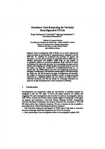
Fig. 9. Layout of the static task (a) and decoder 3 dynamic task (b) on a Virtex XCV800 FPGA.

the synthesis and APR tools. Terminal components are automatically inserted in the necessary locations and layout constraints (expanded from the entries in the RIF file) are added to correctly place the tasks and their terminals. Typically, the design’s external connections are included in the static task. Therefore, the ports in the static design’s entity are converted to IOB pins, while this option is disabled with the dynamic tasks. Within the Foundation APR tools, the option to remove unconnected logic is turned off, to prevent sections of the sub-designs being optimized away. The post-APR layouts for the static task and the (3, 1, 7) dynamic task are shown in Figure 9. SDF and VITALcompliant VHDL descriptions of each dynamic task can optionally be created after APR is complete. DCSTech can be used to post-process these files into a timing model of the overall dynamic design and create a matching RIF file. Configuration bitstreams for each sub-design are created using the Xilinx bitgen tool. As the design contains areas of unconnected logic, the design rule check must be turned off during this process. This stage yields full configurations for each section of the design, which require post-processing into partial configurations. To do this, further information is added to the RIF file to describe which LUT the terminals in each sub-design were mapped to (they were only constrained to a specific slice). In addition, any resources within the dynamic tasks not supported by JBits or JRoute must be replaced be alternative components or settings. DCSBitstream is then used to create activate and deactivate partial configurations for each dynamic task. Back-annotated Timing Simulation and Power Calculation. A backannotated timing simulation can be performed by using DCSim to add simulation components to DCSTech’s post-APR timing model. While DCSim and DCSTech alter the design’s structure and hierarchy, the timing information is unaltered. Consequently the simulation accurately represents the design’s performance. It can be used to check that the design passed through the synthesis and APR stages successfully and to detect serious timing problems. It can also be used as part of the process to calculate the design’s power consumption. The Xilinx XPower tool is used to estimate a design’s power consumption. It requires two inputs: the design .ncd database file (produced during the implementation process) and information on the switching rates of the signals within it. The designer can supply estimates of the switching rates or extract ACM Transactions on Embedded Computing Systems, Vol. 3, No. 2, May 2004.


•

279

Table V. Area Occupation and Maximum Speed of Circuits in the Decoder Design Circuit Static Tasks Decoder 0 Decoder 1 Decoder 2 Decoder 3 RCPC Code

Slices 223 125 478 2,092 2,288 2,530

LUTs 410 225 919 4,066 4,350 4,614

Flip-Flops 308 117 510 2,463 2,556 2,896

Speed (MHz) 46.408 58.394 45.750 40.337 41.135 41.123

them from a back-annotated simulation in a value change dump (.vcd) file. To estimate the power of the dynamic design, the power consumption of each subsection of the design is calculated separately using XPower. Thus, separate .vcd files are required for each subsection. In ModelSim 5.5a the signal activity from different hierarchical subsections of the design can be mapped to different files. Therefore a .vcd file can be created for each dynamic task along with one for the static task. After the simulation, these files indicate the switching activity on each sub-design’s signals during the simulation. Provided the simulation conditions are typical of the design’s operation, these activity levels can be used to estimate its power consumption. The simulation model contains additional signals used to connect the simulation components. The activity on these signals ends up in the .vcd file for the static design. Consequently, the unwanted signals should be removed from the file prior to power calculation. The dynamic tasks are active only part of the time. Therefore, only the sections of their .vcd files relating to their active periods are valid. Any other data should be removed from the file. Simple utilities to perform these tasks were created. 7.2 Comparison of the Reconfigurable and RCPC Code Decoders Table V presents the area occupied by the sections of the reconfigurable design and the programmable RCPC code decoder, along with their maximum operating speed. The static tasks represent circuits that are permanently resident on the logic array. Hence, the area occupied when a dynamic task is active is the sum of its area plus that of the static tasks. The area occupied by this design therefore varies between 348 and 2511 slices. The largest task therefore occupies a comparable area to the programmable RCPC code decoder. In most cases, the area left unoccupied when smaller dynamic tasks are active could not be reused for other circuits, unless run-time floorplanning is used. This typically adds a considerable computational overhead. As expected, the simpler decoder circuits exhibit superior performance to the more complex ones. If the system’s clock speed can be adjusted to match the performance of the dynamic tasks, then its overall performance can be improved, although this is often not easy. However, the static task’s maximum speed, 46 MHz, provides an upper limit to any speed improvements. Unless this can be improved, decoder 0 cannot be run at its full speed. The power consumption of each subsection of the dynamic design and the RCPC code decoder in each of its three modes are shown in Table VI. The ACM Transactions on Embedded Computing Systems, Vol. 3, No. 2, May 2004.

280

•

I. Robertson and J. Irvine Table VI. Estimated Power Consumption in mW of the Subsections of the Dynamic Design and the Static RCPC Code Decoder in Each of its Modes Circuit Static Task Decoder 0 3/4 Decoder 1 1/2 Decoder 2 1/2 Decoder 3 1/3 RCPC 3/4 RCPC 1/2 RCPC 1/3

Quiescent 26.82 26.82 26.82 26.82 26.82 26.82 26.82 26.82

Logic 32.12 50.23 152.61 688.50 864.52 718.35 805.21 895.06

Signal 26.75 21.48 91.23 520.73 641.51 495.47 526.73 567.48

Outputs 2.67 0 0 0 0 0.50 0.50 0.50

Total 88.36 98.52 270.65 1236.04 1532.88 1241.12 1359.24 1489.84

total power consumption of a dynamic task is the task’s power consumption plus that of static circuits. However, each of these figures includes the FPGA’s quiescent power consumption of 26.82 mW. This should therefore be subtracted from the resulting total. Thus, the estimated power consumption of the FPGA with decoder 0 activated is 160 mW. Except for the largest dynamic task, the dynamic circuits consume less power than their programmable alternative. Thus in most modes of operation, the dynamic design consumes less power than the programmable decoder. This analysis only considers the designs after they are configured. To fully determine the power benefits (or otherwise) of the dynamic design, the additional power consumption caused by its reconfigurations should be included. This depends on both the energy consumed during a reconfiguration and the frequency at which they are performed. This in turn depends on the number of error protection levels in the design, the reconfiguration conditions and the behavior of the communications channel. In situations where channel conditions are predominantly good and few reconfigurations are required, substantial power savings will be achieved. However, poor or rapidly varying channel conditions would nullify the benefits. 8. FUTURE WORK While the tools presented in this paper provide the designer with an effective design flow, there are a number of areas in which further research could yield improvements in the tools and their capabilities. Automation of the simulation model extensions presented in Section 3.1, porting these techniques to Verilog and investigating the use of programming language interfaces would improve the generality of the techniques and may improve their run-time efficiency. Increasing numbers of designs, in both ASIC and FPGA, seek to exploit the growing logic capacity of modern devices by integrating many functions onto a single chip. This is known as system-on-a-chip (SoC). The SoC design flow typically contains elements of both hardware and software design. To improve the integration between these previously separate activities, system-level design languages, such as System C and System Verilog, have been developed. These Co-design capabilities are also useful in the design of reconfigurable systems, where both hardware and software can perform computations and control the reconfiguration of areas of the hardware. The application of reconfiguration ACM Transactions on Embedded Computing Systems, Vol. 3, No. 2, May 2004.


•

281

modeling techniques to these languages is therefore important to exploit them effectively in reconfigurable system design. Within the implementation flow, DCSTech currently supports the Virtex and XC6200 FPGAs. Porting to other architectures would further demonstrate its generality. Developing a design management tool, capable of estimating the area requirements of parts of the design and generating placement constraints via a graphical display, could ease the task of floorplanning and partitioning the design. The Virtex-II device includes a self-reconfiguration capability. Porting the configuration port interface for DCSConfig’s configuration controllers would allow automatic generation of configuration controllers for use in selfcontrolling designs on this FPGA. 9. CONCLUSIONS This paper has presented and demonstrated a top-down design flow for partially reconfigurable designs encompassing specification, simulation, synthesis, APR, timing simulation, partial configuration generation and controller design. The majority of the tools and techniques presented are either device independent or easily ported between devices, since they make use of features that are available in the CAD tools for most FPGA platforms. The exceptions are simulation techniques that require changes to the technology libraries for a device (extending the functionality of synchronous components) and the generation of partial configurations. Exploiting the capabilities of programming language interfaces may provide a means of altering the behavior of synchronous components without altering their HDL descriptions. This will make such simulation techniques more portable. The generation of partial configurations relies on access to the configuration data. Such access is not widely available. This, combined with the wide variation in the configuration architecture between devices, means that configuration generation techniques do not port easily between different FPGA families. A reconfigurable Viterbi decoder design was presented. The design allows the error-correcting code used for communication across a fading channel to be adapted according to the prevailing channel conditions. As well as improving utilization of the channel capacity, by adapting the amount of redundancy transmitted, the overall power consumption may be reduced and system performance improved, provided its speed can be adapted in response to reconfigurations. ACKNOWLEDGMENTS

The authors would like to acknowledge the contributions towards the DCS project made by previous members of the DRL research group, in particular Patrick Lysaght, David Robinson, Jon Stockwood and Gordon McGregor. REFERENCES BREBNER, G. 1996. A virtual hardware operating system for the Xilinx XC6200. In Field Programmable Logic and Applications, Darmstadt, Germany, September 1996, R. W. Hartenstein and M. Glesner, eds. Springer-Verlag, Berlin, 327–336. ACM Transactions on Embedded Computing Systems, Vol. 3, No. 2, May 2004.

282

•


BREBNER, G. 1997. CHASTE: A hardware/software co-design testbed for the Xilinx XC6200. In Reconfigurable Architectures Workshop, Geneva, Switzerland, April 1997, R. W. Hartenstein and V. K. Prasanna, eds. IT Press, Verlag, 16–23. CALLAHAN, T. J., HAUSER, J. R., AND WAWRZYNEK, J. 2000. The GARP architecture and C compiler. IEEE Computer 33, 4, 62–69. DANDALIS, A. AND PRASANNA, V. K. 2001. Configuration compression for FPGA-based embedded systems. In 9th ACM International Symposium on Field Programmable Gate Arrays, Monterey, California, USA, February 2001, ACM Press, 173–182. DIANA, L. AND KAHN, J. M. 1999. Rate-adaptive modulation techniques for infrared wireless communications. In Proceedings of the IEEE International Conference on Communications, Vancouver, B. C., Canada, June 1999, 597–603. DYER, M., PLESSL, C., AND PLATZNER, M. 2002. Partially reconfigurable cores for Xilinx virtex. In Field Programmable Logic and Applications, Montpellier, France, September 2002, M. Glesner, P. Zipf, and M. Renovell, eds. Springer-Verlag, Berlin, 292–301. FAURA, J., MORENO, J. M., MADRENAS, J., AND INSENSER, J. M. 1997. VHDL modelling of fast dynamic reconfiguration on novel multicontext RAM-based field-programmable devices. In Proceedings of the SIG-VHDL Spring’97 Working Conference, Toledo, Spain, April 1997, 171–177. GOKHALE, M. B., STONE, J. M., ARNOLD, J., AND KALINOWSKI, M. 2000. Stream-oriented FPGA computing in the streams-C high level language. In Proceedings of the Eighth Annual IEEE Symposium on Field-Programmable Custom Computing Machines (FCCM), Napa, California, USA, April 2000, K. L. Pocek and J. Arnold, eds. IEEE Computer Society Press, 49–56. GOLDSMITH, A. J. AND CHUA, S. G. 1998. Adaptive coded modulation for fading channels. IEEE Trans. Commun. 46, 5, 595–602. GUCCIONE, S., LEVI, D., AND SUNDARARAJAN, P. 1999. JBits: Java-based interface for reconfigurable computing. In Military and Aerospace Applications of Programmable Devices and Technologies Conference, Laurel, MD, September 1999. HAGENAUER, J. AND STOCKHAMMER, T., 1999. Channel coding and transmission aspects for wireless multimedia. Proc. IEEE 87, 10, 1764–1777. HORTA, E. L., LOCKWOOD, J. W., TAYLOR, D. E., AND PARLOUR, D. 2002. Dynamic hardware plugins in an FPGA with partial run-time reconfiguration. In Proceedings of the 39th Design Automation Conference, Los Angeles, USA, June 2002, 343–348. HUTCHINGS, B., NELSON, B., AND WIRTHLIN, M. J., 2000. Designing and debugging custom computing applications. IEEE Design and Test of Computers 17, 1, 20–28. KELLER, E. 2000. JRoute: A run-time routing API for FPGA hardware. In The Seventh Reconfigurable Architectures Workshop, Cacun, Mexico, May 2000, J. Romlin, ed. Springer-Verlag, Berlin, 874–881. KWIAT, K. AND DEBANY, W. 1996. Reconfigurable logic modelling. Integrated System Design (Dec.). LI, Y., CALLAHAN, T., DARNELL, E., HARR, R., KURKURE, U., AND STOCKWOOD, J., 2000. Hardware– software codesign of embedded reconfigurable architectures. In Proceedings of the 37th Design Automation Conference, Los Angeles, USA, June 2000, 507–512. LUK, W. AND MCKEEVER, S. 1998. Pebble: A language for parameterised and reconfigurable hardware design. In Field Programmable Logic and Applications, Tallinn, Estonia, September 1998, R. W. Hartenstein and A. Keevallik, eds. Springer-Verlag, Berlin, 9–18. LYSAGHT, P. AND STOCKWOOD, J. 1996. A simulation tool for dynamically reconfigurable field programmable gate arrays. IEEE Trans. VLSI Syst. 4, 3, 381–390. MACBETH, J., 2003. Dynamically Reconfigurable Intellectual Property Cores (DRIP Cores). Ph.D. Thesis, University of Strathclyde, UK. MCKAY, N. AND SINGH, S. 1999. Debugging techniques for dynamically reconfigurable hardware. In IEEE Symposium on Field-Programmable Custom Computing Machines, Napa, California, USA, April 1999, K. L. Pocek and J. Arnold, eds., IEEE Computer Society Press, 114–122. MCMILLAN, S. AND GUCCIONE, S. 2000. Partial run-time reconfiguration using JRTR. In Field Programmable Logic and Applications, Villach, Austria, August 2000, R. W. Hartenstein and H. Grunbacher, eds. Springer-Verlag, Berlin, 352–360. MCMILLAN, S., BLODGET, B., AND GUCCIONE, S. 2000. VirtexDS: A device simulator for Virtex. Reconfigurable Technology: FPGAs for Computing and Applications II. Proc. SPIE 4212, Bellingham, WA, November 2000. ACM Transactions on Embedded Computing Systems, Vol. 3, No. 2, May 2004.


•

283

PANDITA, B. AND ROY, S. K., 1999. Design and implementation of a Viterbi decoder using FPGAs. In 12th International Conference on VLSI Design, Goa, India, January 1999, 611–614. ROBERTSON, I., IRVINE, J., LYSAGHT, P., AND ROBINSON, D. 2002a. Timing verification of dynamically reconfigurable logic for the Xilinx Virtex FPGA series. In Tenth ACM International Symposium on Field-Programmable Gate Arrays, Monterey, California, USA, February 2002, M. Schlag and S. Trimberger, eds. ACM Press, 127–135. ROBERTSON, I., IRVINE, J., LYSAGHT, P., AND ROBINSON, D. 2002b. Improved functional simulation of dynamically reconfigurable logic. In Field Programmable Logic and Applications, Montpellier, France, September 2002, M. Glesner, P. Zipf, and M. Renovell, eds. Springer-Verlag, Berlin, 152– 161. ROBINSON, D. 2002. Simulation and Control of Dynamically Reconfigurable Logic Circuits. Ph.D. Thesis, University of Strathclyde, UK. ROBINSON, D. AND LYSAGHT, P. 2000a. Methods of exploiting simulation technology for simulating the timing of dynamically reconfigurable logic. IEE Proc. Comput. Digital Tech. 147, 3, 175–180. ROBINSON, D. AND LYSAGHT, P. 2000b. Verification of dynamically reconfigurable logic. In Field Programmable Logic and Applications, Villach, Austria, August 2000, R. W. Hartenstein and H. Grunbacher, eds. Springer-Verlag, Berlin, 141–150. SHIRAZI, N., LUK, W., AND CHEUNG, P. Y. K. 1998. Automating production of run-time reconfigurable designs. In Proceedings of the Sixth Annual IEEE Symposium on Field-Programmable Custom Computing Machines, Napa, California, USA, April 1998, K. L. Pocek and J. Arnold, eds. IEEE Computer Society Press, 147–156. SINGH, S. AND JAMES-ROXBY, P. 2001. Lava and JBits: From HDL to bitstream in seconds. In Proceedings of the Ninth Annual IEEE Symposium on Field-Programmable Custom Computing Machines, Rohnert Park, California, USA, April 2001, K. L. Pocek and J. Arnold, eds. IEEE Computer Society Press. SWAMINATHAN, S., TESSIER, R., GOECKEL, D., AND BURLESON, W. 2002. A dynamically reconfigurable adaptive Viterbi decoder. In Tenth ACM International Symposium on Field-Programmable Gate Arrays, Monterey, California, USA, February 2002, M. Schlag and S. Trimberger, eds. ACM Press, 227–236. TRIMBERGER, S. 1998. Scheduling designs into a time-multiplexed FPGA. In Sixth ACM International Symposium of Field Programmable Gate Arrays, Monterey, California, USA, February 1998, ACM Press, 153–160. TRIPP, J. L., JACKSON, P. A., AND HUTCHINGS, B. L. 2002. Sea cucumber: A synthesizing compiler for FPGAs. In Field Programmable Logic and Applications, Montpellier, France, September 2002, M. Glesner, P. Zipf, and M. Renovell, eds. Springer-Verlag, Berlin, 875–885. VASILKO, M. 1999. DYNASTY: A temporal floorplanning based CAD framework for dynamically reconfigurable logic systems. In Field Programmable Logic and Applications, Glasgow, UK, August 1999, P. Lysaght, J. Irvine and R. W. Hartenstein, eds. Springer-Verlag, Berlin, 124–133. VASILKO, M. AND CABANIS, D. 1999. A technique for modelling dynamic reconfiguration with improved simulation accuracy. IEICE Trans. Fundam. Electron., Commun. Comput. Sci. E82 − A, 11, 2465–2474. XILINX, INC. 2002. XAPP290: An Implementation Flow for Active Partial Reconfiguration Using 4.2i, Application Note, version 0.7, March 2002. YANG, J., KHANDANI, A. K., AND TIN, N. 2002. Adaptive Modulation and Coding in 3G Wireless Systems. Technical Report UW-E&CE#2002-15, University of Waterloo, Waterloo, Ontario, Canada. YEH, D., FEYGIN, G., AND CHOW, P. 1996. RACER: A reconfigurable constraint-length 14 Viterbi decoder. In Proceedings of the IEEE Symposium on Field-Programmable Custom Computing Machines, Napa, California, USA, April 1996, K. L. Pocek and J. Arnold, eds. IEEE Computer Society Press, 60–69. Received January 2003; revised June 2003; accepted August 2003

ACM Transactions on Embedded Computing Systems, Vol. 3, No. 2, May 2004.