Resources are managed by software agents. ... solution guarantees the discovery of the best global solu- ... gate knowledge a, the agent chooses the best plan.
A Distributed Agent-based Approach to Stabilization of Global Resource Utilization Evangelos Pournaras Martijn Warnier Frances Brazier Intelligent Interactive Distributed Systems VU University, Amsterdam The Netherlands {E.Pournaras,M.Warnier,FMT.Brazier}@few.vu.nl
Abstract Distributed management of complex, distributed systems is the focus of this paper. Adaptation through local deliberation by software agents within a hierarchical virtual organization is the approach taken. Global stabilization of resource utilization is the goal. Electricity networks are used to illustrate the potential of two fitness functions on the basis of which local choices for resource utilization are made: minimizing oscillations is the first function considered, reversing oscillations the second. Results reveal considerable increase in the stabilization of resource utilization compared to a system that utilizes resources in a greedy manner.
1. Introduction Complex, intelligent, distributed systems in dynamic environments need to adapt continually. Central management of such systems is not often an option: distributed management is required. This paper addresses distributed management of resource utilization. Resources are managed by software agents. Software agents are capable of reasoning with and about (1) their own knowledge at any given time, (2) knowledge they receive from other agents and (3) knowledge they acquire from interaction with their environment, with respect to their goals. They act accordingly, adapting to change as required. Note that adaptivity has been recognized as a means to handle arising complexity of knowledge and interactions [14]. Virtual organizations of agents define communication structures between agents, e.g., hierarchical organizations [4], between and within which agents can choose to cooperate and coordinate their actions, or compete. Dynamic organized hierarchies [9] can be used to support adaptive, aggregate, nonlinear behavior, as a means to re-
duce complexity. Coordination in unstructured environments entails distributed search and distributed scheduling [13, 5]. This paper proposes a fully decentralized agent-based approach to global stabilization of resource utilization, based on local coordination. The core question addressed is: To which extent can global stabilization in resource utilization be acquired by local coordination of resource utilization using software agents to manage resources? The approach is threefold and can be outlined as follows: 1. Agents are members of a hierarchical virtual organization, structuring agent interactions and aggregation of agent resource requirements. 2. A simple agent knowledge model is assumed on the basis of which resource requests are generated. 3. Agents can make local adaptive decisions on the basis of information they receive from the agents to which they are linked. The problem and the proposed solution are illustrated in the context of the electricity domain. In this context, global stabilization is acquired in the energy consumption of an electricity network. In particular, this paper focuses on minimizing the oscillations of thermostatic controlled appliances. These devices, (e.g. refrigerators, air conditioners, water heaters) consume 25% of the total energy supply in the USA [10], thus management of these devices can have a significant effect on the stabilization of global resource consumption. Software agents can autonomously negotiate their resource requirements and configuration [3, 2]. Based on the above application domain, a network of interconnected software agents representing thermostatic devices has been designed, developed and implemented/simulated. Agents interact and use local knowledge on the basis of which they make local adaptive decisions
towards stabilizing the global consumption. Two different algorithm variations have been examined: (i) one that aims to achieve minimum oscillations in each and every aggregation round and, (ii) one that reverses oscillations with respect to a previous aggregation round (to acquire the opposite deviation values). This results in global stabilization over a series of aggregation rounds. The first variation shows considerable improvement in the global stabilization compared to a greedy system that makes random resource utilization choices from the set of its alternative utilization options. The second algorithm variation achieves almost constant utilization with minimum oscillations over time.
various factors, including a number of uncertainties [8] in user consumption, influenced by the characteristics of individual devices and the environments in which the devices operate. This paper assumes that the utility functions used by agents to devise alternative plans for resource utilization, take these uncertainties into account, see [6, 7]. These plans denote the options for energy consumption, i.e., the distribution of consumption, over a fixed period of time. Finally, the on/off state of the thermostat is configured by temperature setpoints. Modifying the temperature creates equivalent operational states for the device [1]. These states are the possible plans that the agents can generate.
2. The Distributed Coordination Environment
3. The Locality of the Agents
This paper assumes a distributed environment with software agents representing thermostatic devices that manage their behavior. Agents reason about resource utilization within a given period of time, generating alternative distributions of resource utilization within this period, with equivalent effect. In this paper, these alternative utilization distributions are called possible plans. The most straightforward solution to the above problem is to centrally combine and aggregate all possible plans for all of the agents, and to choose the best combination. This solution guarantees the discovery of the best global solution, considering and assuming that the sets of possible plans do not change during aggregation. Central aggregation, however, does not scale. The complexity is O(pn ), where p is the number of possible plans per agent and n is the number of agents in the network. In contrast, the challenge in distributed solutions is to perform distributed computation and decision making in a cost-effective manner. The solution this paper proposes is to stabilize global utilization by decentralized energy plan aggregation within a hierarchical virtual structure. In this case, complexity is bounded to O(pc ) where c is the number of children per node in the hierarchical structure. The estimations assume a balanced hierarchical structure, i.e., a tree structure, and fixed p for all agents. Scalability improves significantly and it is influenced by the trade-off between processing cost and latency. The hierarchical structure minimizes communication overhead. Each node receives one message from each of its children, and one message from its parent during each aggregation round. The problem of robustness can be overcome by building reliability-driven hierarchical structures, i.e., trees. In this approach, more reliable nodes move up in the tree, leaving unreliable ones underneath to minimize the effect of failure. Although this paper does not focus on the issue of tree robustness, various mechanisms can be used to guarantee a relatively stable tree [12]. The resource utilization profile of an agent depends on
Agents use local knowledge to perform local computations and execute their tasks locally, using knowledge acquired from their children and/or their parent.
3.1. Overview of Agent Tasks The main tasks of an agent are (plan) generation, (plan) aggregation and (plan) execution: Generation is composed of two subtasks: • Planning: A set P of possible plans p is generated for the energy consumption of the thermostatic device that an agent represents over a fixed time period. • Parent Inform: The agent sends its possible plans P and its aggregate knowledge a to its parent. The aggregate knowledge is described in detail in Section 3.2. Aggregation is composed of three subtasks: • Selection: Upon receiving the sets of possible plans P from each of its children together with the aggregate knowledge a, the agent chooses the best plan combination c0 ∈ C according to a fitness function f (C, A, h). The fitness function receives as input the set C with all the unique combinations c of plans derived from the possible plans p received from each of the children. The computation of C is illustrated in Section 3.3. It also receives the set A of each of its children’s aggregate knowledge a and the history knowledge h that is locally retained. The history h is described in detail in Section 3.2. • Update: The agent’s aggregate knowledge a is updated as update(c0 , A, h). More information about the update task is given in Section 5.1 and 5.2. • Children Inform: The agent sends the selected plans p0 to its children.
Execution concerns the execution of the selected plan p0 ∈ P that has been received from the parent. The root agent executes an additional broadcast task that is important for the aggregation process. Section 4 provides more information about the execution of this additional task.
starts when a ’parent-inform’ is received by an agent and is outlined by the sequence of tasks executed as illustrated in Algorithm 1 below.
3.2. Aggregate and History Knowledge The aggregate knowledge a = (an , ah ) represents the selections of a set of agents that have been made so far. It includes: the aggregate new plan an and the aggregate history plan ah . The latter is the plan that represents the selections of the respective agents in the previous aggregation. Note that p0 ∈ h ⊆ ah ⊆ g ∈ h. The aggregate knowledge a known to leaf agents is zero, whereas the aggregate knowledge of the root agent, at the end of each round, is the final converged global plan. The notion of history h as part of each agent’s knowledge is, in fact, a set h = (p0 , g) that includes: (i) the most recently selected plan p0 ⊂ g ∈ h and (ii) the root’s aggregate plan, that is the global plan g as a result of an aggregation round. This plan is broadcasted by the root at the end of each round. The broadcast task is illustrated in Section 4.
3.3. Pre-Processing of the Local Knowledge Before an agent can calculate the fitness function, it performs some pre-processing of the information it receives from its children. This pre-processing concerns the computation of all possible combinations C of all possible plans received from its children. For example, an agent with 2 children, each with 2 possible plans will generate the following 4 combinations:
Figure 1. A generic agent ‘A’ that performs the core agent algorithm Algorithm 1 Core agent algorithm if receive parent inform and is not root then aggregation-selection; aggregation-update; aggregation-children inform; generation-planning; generation-parent inform;
The leaf agents and the root agent have a special role during an aggregation round. The leaf agents wait for a broadcast message to initiate the aggregation process by executing the two ‘generation’ subtasks in order. The root agent selects its own execution plan, without sending the plans to another agent. In this case, the set of combinations is C = P . In other words, the root aggregates twice, one for its children and one for itself. Moreover, the root broadcasts information to all the other agents and initiates the next aggregation round. Two levels of aggregation are distinguished in the aggregation process : The aggregation step and the aggregation round. Figure 2 illustrates these two concepts.
C = {(P 11 + P 21 ), (P 11 + P 22 ), (P 12 + P 21 ), (P 12 + P 22 )} with the expression P child plan defining the plans in every combination. Each agent also merges the aggregate knowledge received from its children by summing up the respective aggregate plans. The aggregate knowledge is merged as follows: a={
X i=1,2,...,|A|
an ∈ Ai ,
X
ah ∈ Ai }
(1)
i=1,2,...,|A|
4. The Aggregation Process The core agent algorithm for each (non-root) agent ‘A’ with children ‘C1’,‘C2,’,... and a parent ‘P’ (see Figure 1)
Figure 2. The aggregation step and aggregation round An aggregation step is defined by the core agent execution process described above for each agent within the same level in the hierarchical structure. Given input from its children, each agent within the same level of the hierarchical structure aggregates the information and sends results to its parent and to its children. The procedure recurses, starting from the leaf agents up to the root agent.
An aggregation round is defined by all of the consecutive aggregation steps starting from the leaf agents up to the root agent, ending with the global aggregate plan g being broadcasted to all agents. When the leaf agents receive the broadcast message, the next aggregation round is triggered. Alternatively, although not discussed in this paper, a next aggregation round can start independently by the leaf agents. In this case, multiple aggregation round may run simultaneously over the hierarchical structure.
5. Fitness Function The fitness function forms the core of the adaptivity and decision making of the agents. This function is used by agents for the selection of the best combination. Two different fitness functions have been devised, implemented and evaluated. The goal of both fitness functions is to stabilize resource utilization over time.
5.1. Stabilization by Minimizing Deviations The simplest fitness function defines the best combination c0 to be the combination that minimizes the standard deviation σ of the aggregate new plan an . In this stabilization scenario, the fitness function can be expressed as:
fMD =
min i=1,2,...,|C|
σ(an + C i )
(2)
This fitness function checks which of the potentially new aggregate plans has the minimum overall standard deviation σ. Section 6 discusses the convergence of the process. The selected plans for every child are extracted from the best combination c0 . Moreover, the aggregate knowledge is updated. This action concerns the update of the aggregate new plan as an = an + c0 . Finally, the selected plans are sent to the respective children.
5.2. Stabilization by Reversing Deviations The second fitness function averages out the global resource utilization between aggregation rounds, by reversing deviations in an existing global plan. This history global plan was devised by the same agents, representing the same devices in the same virtual structure. This fitness function specifies that, if resource providers have to supply g + vt amount of resources at time t, the reverse of the deviations provides g − vt . vt is the difference between the average value g and the value of the global plan at time t. The aggregation process remains exactly the same. The fitness function is calculated as follows:
history
fRD
new
z }| { z }| { = min σ(g − ah +an + C i ) i=1,2,...,|C| | {z }
(3)
replacement
The aggregate history ah is replaced by the equivalent summation of the aggregate new plan an and the plan C i from the combinations (ah ≡ an + C i ). This replacement is adapted to the global plan g ∈ h. The concept of this reversing operation is the following: The average of the global history plan and global new plan must ideally result in zero deviations. This is because (g+vt )+(g−vt ) = g. Choosing the combination that con2 tributes best on transforming vt to −vt results in a global plan with reversed deviations. The transformation is gradually achieved in every aggregation step. Section 6 discusses the convergence of this process. Finally, as in the previous scenario, the aggregate knowledge is updated as a = {(an = an + c0 ), (ah = ah + p0 ∈ h)}. As mentioned in Section 5.1, the selected plans are extracted and sent to the respective children.
6. Emerging Stabilization Convergence The two fitness functions described in Section 5.1 and 5.2 are based on local knowledge. The decisions each agent makes are based on the aggregate plans it receives from its children, by definition an incomplete version of the global knowledge. Summations are performed over the hierarchical structure during the aggregation process. In each aggregation step, the aggregate values of the aggregate plans increase. As a result, the combinations are adapted to plans that come from the operations of more agents. The aggregation starts from the leaf agents. The parents provide the best solution taking into account the information from children. The aggregate knowledge is zero. In the next steps, local decisions have a twofold advantage. Each agent not only chooses the plans (1) that satisfy the stabilization goal locally but also (2) plans that ‘fade out’ the effect of less optimal decisions in previous aggregation steps. For the first fitness function, the approach based on minimizing deviations, the second advantage is achieved by adapting the combinations to the aggregate new plan. For the second fitness function, the approach based on reversed deviations, the aggregate history plan is replaced by the aggregate new plan and adapted to the global history plan. The effect of adaptation increases after each aggregation step. This step-by-step emerging convergence is depicted in Figure 3 for the second fitness function, namely the function based on reversed deviations. In the first aggregation steps, decisions are mainly based on the history plan. As aggregation evolves, the global history plan is gradually replaced by the aggregate new plans. Finally, the aggregate
new plan converges to the new global plan devised by the root agent.
Section 7.1 outlines the simulation environment and Section 7.2 and 7.3 illustrate the results for the two stabilization actions.
7.1. Simulation Environment The simulation scenario assumes a network of interconnected thermostatically controlled appliances. These devices are represented by software agents in a hierarchical virtual structure. The hierarchical structure, that is a tree, is balanced. The heterogeneity of devices over the network is simulated by a top-down approach illustrated in Figure 4 below.
Figure 3. Step-by-step aggregation and stabilization convergence using reversed deviations.
7. Experiments and Results This section illustrates the experimental environment and the results of the stabilization approach. More specifically, the two fitness functions described in Section 5.1 and 5.2 are applied to two energy management scenarios: oscillations minimization and oscillations reverse. The goal of the experiments is to reveal how a system that coordinates multiple utilization plans locally outperforms a fitness function in which an agent’s choice of plans is based on random selection. The experimental study aims to answer the three following questions: 1. What is the degree of oscillation minimization achieved in the hierarchical structure compared to random plan selection and centralized coordination? 2. What is the degree of successful reversed oscillations? 3. How does the number of possible plans influence the effect of the two fitness functions in a hierarchical structure?
Figure 4. The top-down approach of the simulation environment configuration The simulation configuration starts by considering the following (Level 1 in Figure 4): (i) the average consumption of a generic thermostatically controlled appliance, (ii) the deviation of this average consumption that provides different types (refrigerator, water heater etc.) of thermostatic devices and (iii) the total number of these types. Then a number of average consumption seed values for every type of device are randomly generated (Level 2 in Figure 4). The seed values belong to the range defined by the deviation of average consumption that provides different types of thermostatic devices. The number of seeds is equal to the number of types of thermostatically controlled appliances in the network. The consumption of a specific type of device also varies in much smaller proportion compared to the deviation of average consumption among different types (Level 3 in Figure 4). Moreover, every agent in the network, regardless of which type of device it represents, generates a fixed number of possible plans over a fixed time period (Level 4 in Figure 4). The generation of the plans is simulated as follows: for every final average consumption of every device,
a random sample is generated with size equal to the number of energy values of the plan. The values are estimated between a percentage range of plan deviation from the average consumption value of the plan. For example, a 20% plan deviation from the average consumption of value 10, results in deriving the random value from the range [8,12]. Finally, user consumption profiles are simulated (Level 5 in Figure 4). Each device has a high, a medium and a low consumption profile. A consumption profile coefficient multiplies or divides respectively the values of the possible plans. The profiles change cyclically in every round and they are initially attributed randomly between devices. This means that every individual device may start with any of the high, medium and low consumption profiles and it will follow the same cyclical row in every round. There are two simulation environments. The first simulation environment is a small-scale system with 15 agents, each with 2 possible plans. This environment is used for running the centralized coordination as the central coordination of 3280 agents does not scale. The second environment represents a large-scale distributed system with 3280 agents with every agent generating 5 possible plans. Most of the experiments are performed in this environment. Table 1 outlines the parameters for each of the simulation environments. Table 1. Simulation environments Parameter SE 1 Num. of Agents 15 Num. of Children 2 Num. of Possible Plans 2 Num. of Values/Plan 10 Avg. Device Consumption 0.5 Num. of Device Types 3 Avg. Cons. Deviation/Type 0.35 Avg. Cons. Deviation/Type/Device 0.035 Plan Deviation 90% Num. of Consumption Profiles 3 Consumption Profile Coefficient 2
SE 2 3280 3 5 10 0.5 3 0.35 0.035 90% 3 2
Figure 5. Stabilization comparison of hierarchical coordination vs. random plan selection and central coordination in the ‘SE 1’ The comparison in this small-scale environment indicates that the proposed method outperforms random plan selection and is not far from the optimal centralized coordination. The average standard deviation for 100 rounds in the centralized solution is 0.42, in hierarchical aggregation and random plan selection the standard deviation is 0.79 and 1.08 respectively. Figure 6 illustrates the energy consumption of 3 consecutive global plans that consist of 30 time intervals. In every round, or every 10 time intervals, the consumption changes due to the individual profiles. Note that the normalization of the global consumption is higher and closer to the average. The oscillations decrease 78.71%, 36,54% and 73.46% in the respective coordinated global plans compared to the random plan selection. This difference in the global plans is depicted in the three enlarged figures.
Note that the units for energy consumption are the same in both environments.
7.2. Oscillations Minimization The oscillations minimization corresponds to the minimum deviations fitness function. The stabilization is evaluated by calculating the standard deviation of the final plans at the end of each round. Figure 5 shows a stacked bar chart with a comparison of the stabilization effect between the proposed hierarchical aggregation, the central coordination and the random plan selection.
Figure 6. The global energy consumption of hierarchical coordination and random plan selection in the ‘SE 2’ during 3 rounds Please note that the proposed stabilization method does not aim to stabilize consumption between different profiles.
The global energy consumption changes and this paper focuses on the decrease of positive and negative peak loads in the aggregate plans. Finally, the effect of increasing the number (#) of possible plans in standard deviation is illustrated in Figure 7. The values are the average ones of 30 simulation rounds for each of the 3 consumption profiles (90 rounds in total). The values of the profiles are also averaged for each method and depicted with the thicker solid lines.
Figure 8. The reverse effect between the history and new plan in ‘SE 2’ approaches ‘-1’, perfect reversing has been achieved. Figure 9 illustrates how the increase in the number (#) of possible plans results in a better negative correlation.
Figure 7. The change in the standard deviation of the global plans in ‘SE 2’ as the number of possible plans increases The increase in the number of possible plans influences the stabilization positively. For 2 possible plans the difference between the two methods is 9.41, whereas for 7 possible plans it almost doubles to 17.96, denoting almost double improvement. The reason for this positive influence is the increased number of options from which agents can choose, resulting in a higher potential for better stabilization.
7.3. Oscillations Reverse The oscillations reverse corresponds to the reverse oscillations fitness function. The evaluation focuses on how well the aggregate new plan reverses the aggregate history plan. This means that, ideally, the average of these two must be a plan with zero deviations, resulting in a flat global energy consumption. Figure 8 illustrates three global energy plans that correspond to the different consumption profiles. The global new plan converges to a mirroring version of the global history plan. The average of these two plans is also drawn to depict the effect of the flat energy consumption. The number of possible plans also influences the reversing effect. In this case, the similarity between the history and new global plan has been examined by increasing the number of possible plans in each agent. Similarity is measured by calculating the correlation coefficient r of the values of the plans. If the value of the correlation coefficient
Figure 9. Negative correlation of the global plans in ‘SE 2’ as the number of possible plans increase
7.4. Evaluation Summary The results in the two simulation environments depicted in Table 1 provide the following answers to the questions set at the beginning of this section: 1. What is the degree of the minimum oscillations achieved in hierarchical coordination compared to random plan selection and centralized coordination? Hierarchical coordination always provides higher stabilization than random plan selection. In the largescale experimental environment, oscillations decrease in the range of 36.54%-78.71%. The smaller-scale experimental environment indicates stabilization of hierarchical coordination (0.79) between central coordination (0.42) and random plan selection (1.08).
2. What is the degree of the successful oscillations reverse? The reversed plans approach the maximum possible negative correlation. The correlation coefficient approaches ‘-1’. The average result of the two plans corresponds to a flat stabilized plan with its oscillations approaching zero. 3. How does the number of possible plans influence the effect of the two stabilization functions? The increase in the number of possible plans increases the stabilization in both fitness functions. In the minimum oscillations, the improvement between hierarchical coordination and random plan selection almost doubles. In oscillations reverse, the negative correlation increases to approach ‘-1’. These achievements come together with a bounded processing cost to the number of children of every node.
8. Conclusions and Future Work This paper describes a method of global stabilization of resource utilization, by local coordination. More specifically, agents provide alternative options, aggregate information, choose utilizations and communicate over a hierarchy. The main contribution of the proposed approach is the following: Hierarchical local coordination achieves emerging convergence of the global stabilization through local knowledge, local decisions and local interactions by individual software agents. This paper describes the stabilization problem in the context of the electricity domain. It shows how the requirements of the proposed method fit with the requirements of electricity suppliers for minimizing oscillations in energy consumption. The results for two different fitness functions reveal a considerable improvement compared to a system that randomly chooses utilizations to satisfy its own goals. The hierarchical organization can influence the effect of the proposed method. Thus, future work should shed light on how the number of children, the number of levels in the hierarchical structure and the failures affect the global stabilization and the performance of the aggregation. Work on extending the results to simulations in an asynchronous communication environment is in progress. Experiments will run on the AgentScape [11] platform, a middleware system that supports large-scale agent systems.
Acknowledgments This project is supported by the NLnet Foundation http://www.nlnet.nl.
References [1] Y. Guo, J. Li, and G. James. Evolutionary optimisation of distributed energy resources. In Australian Conference on Artificial Intelligence, pages 1086–1091, 2005. [2] D. Hammerstrom. Part II. Grid FriendlyTM Appliance Project. PNNL 17079, Pacific Northwestern National Laboratory, October 2002. [3] G. James, D. Cohen, R. Dodier, G. Platt, and D. Palmer. A deployed multi-agent framework for distributed energy applications. In 5th International Joint Conference on Autonomous Agents and Multi-agent Systems (AAMAS 2006),Hakodate, Japan, May 2006. [4] N. R. Jennings. An agent-based approach for building complex software systems. Commun. ACM, 44(4):35–41, 2001. [5] S. Johansson, P. Davidsson, and B. Carlsson. Coordination models for dynamic resource allocation. In Coordination Models and Languages, pages 182–197, 2000. [6] S. Lefebvre and C. Desbiens. Residential load modeling for predicting distribution transformer load behavior, feeder load and cold load pickup. International Journal of Electrical Power and Energy Systems, 2002. [7] N. Lu, D. P. Chassin, and S. E. Widergren. Simulating price responsive distributed resources. In Power Systems Conference and Exposition, October 2004. [8] N. Lu, D. P. Chassin, and S. E. Widergren. Modeling uncertainties in aggregated thermostatically controlled loads using a state queueing model. IEEE Transactions on Power Systems, 20(2), 2005. [9] M. Luis. Complex system modeling: Using metaphors from nature in simulation and scientific methods. BITS: Computer and Communications News, Computing, Information and Communications Divisions, November 1999. Available online via: http://www.c3.lanl.gov/ rocha/complex/csm.html (accessed September 30, 2008). [10] P. Mazza. The smart energy network: Electrical power for the 21st century. Climate Solutions, 2002. [11] B. J. Overeinder and F. M. T. Brazier. Scalable middleware environment for agent-based internet applications. In Proceedings of the Workshop on State-of-the-Art in Scientific Computing (PARA’04), volume 3732 of Lecture Notes in Computer Science, pages 675–679, Copenhagen, Denmark, June 2004. Springer. [12] G. Tan, S. A. Jarvis, and D. P. Spooner. Improving the fault resilience of overlay multicast for media streaming. In DSN ’06: Proceedings of the International Conference on Dependable Systems and Networks, pages 558–567, Washington, DC, USA, 2006. IEEE Computer Society. [13] C. Theocharopoulou, I. Partsakoulakis, G. A. Vouros, and K. Stergiou. Overlay networks for task allocation and coordination in dynamic large-scale networks of cooperative agents. In AAMAS ’07: Proceedings of the 6th international joint conference on Autonomous agents and multiagent systems, pages 1–8, New York, NY, USA, 2007. ACM. [14] M. Wirsing and M. Holzl. Software intensive systems. Technical report, Beyond the Horizon Thematic Group 6 on Software Intensive Systems, 2006.