A DISTRIBUTED APPROACH TO GLOBAL SEMANTIC LEARNING ...

3rd International Conference “From Scientific Computing to Computational Engineering 3rd IC-SCCE Athens, 9-12 July, 2008 © IC-SCCE

A DISTRIBUTED APPROACH TO GLOBAL SEMANTIC LEARNING OVER A LARGE SENSOR NETWORK C. Picus1, L. Cambrini1, W. Herzner1, D. Bruckner* and G. Zucker* 1

Austrian Research Centers (ARC) A-1220 Vienna, Austria e-mail: {cristina.picus|luigi.cambrini|wolfgang.herzner}@arcs.ac.at *

Vienna University of Technology, ICT A-1040 Vienna, Austria e-mail: {bruckner|zucker}@ict.tuwien.ac.at Keywords: distributed sensor networks, embedded sensors, collaborative learning, semantic processing. Abstract. Sensor networks play an increasing role in several disciplines like security surveillance or environmental monitoring. A challenge of such systems is integration of observations from individual nodes into a common semantic representation of their environment. In this paper, an approach for establishing such a global view is presented, solely by correlating local information learned at the level of each sensing unit. Each node has two modes of processing environment information: it learns the “usual” events and “objects“ in its environment by means of probabilistic methods and it uses a set of predefined rules to detect standard situations that are uncommon or possibly dangerous. In the ongoing implementation of a security surveillance system, models of local activity at each node are inferred by processing video and audio data from its sensors, which are, for our test application, a camera and a microphone array. A local processing stack at each node serves to reduce spurious data from the sensors, to learn typical behavior and to detect unusual behavior by means of statistical techniques as well as predefined alarm situations by means of rule-based approaches. Communication with the neighbor nodes by means of a wireless network is used to build a shared understanding of the environment. The correlations of events and modalities among nodes are learned in order to establish neighborhood correspondences. The shared knowledge between neighbor nodes is used to enrich the local description of the learned normality. This can be used to establish paths over sensing zone boundaries of individual nodes, obtaining inter-node trajectories of observed objects. In addition, this approach avoids the necessity of precise calibration of the individual nodes. 1

INTRODUCTION

Embedded computer systems have seen their computing power increase dramatically, while at the same time miniaturization and wireless networking allow embedded systems to be installed and powered with a minimum of support infrastructure. The result has been a vision of “ubiquitous computing”, where computing capabilities are always available, extremely flexible and support people in their daily lives. Dedicated application areas are security surveillance [7], home care [9], environmental monitoring [10], or smart buildings [2] [5]. Although hardware and networking capabilities have increased dramatically, one necessary piece of technology for ubiquitous computing has generally lagged behind. The intelligent middleware embedded in smart devices for resource discovery, adaptive configuration, flexible cooperation and high-level perception has not kept pace with hardware advances. Some strides in this direction have been made [4], but perception and adaptation are current topics in robotics and artificial intelligence, as resource discovery and dynamic networking are active topics of research in embedded systems. In particular, minimizing the configuration and calibration effort of such systems emerges as requirement whose fulfillment is critical for their industrial acceptance and economic success. In awareness of that situation, the European project SENSE (Smart Embedded Network of Sensing Entities) 1 targets to combine these two aspects in a common framework of semantic knowledge discovery and sharing. Seeing the task of adaptation as a learning process, the SENSE approach is based on machine learning concepts. Further, recognizing that centralized solutions – though attractive due to their simplicity and hence repeatedly adopted as underlying architecture – carry the risk of putting limitations on both size and complexity of sensor 1

SENSE is co-funded by the European Commission under contract No. 033279 within framework programme 6

First A. Author, Second B. Author, and Third C. Coauthor.

networks with respect to communication and computational resources, as well as of raising vulnerability against faults in central parts, SENSE takes a decentralized approach. A sensor network consists of a number of identical, autonomous acting entities, or nodes. Each node possesses sensors - in our test application these are cameras and microphone arrays - gathers information from its surroundings, and interprets it. Consequently, each node can be seen as a stand alone system. However, the nodes are able to share that knowledge with their neighboring nodes. Each node acquires knowledge not just from its own sensors, but from its neighbors, and integrates this knowledge into its own world view. In this way, a global world view is created autonomously. These principles are illustrated in figure 1. Communication within SENSE takes place only between neighboring nodes, and computation is local. This enables scalability. The breakdown or removal of a node will have only a slight, temporary effect on neighboring nodes, besides the absence of local observations provided to the user interface. A condition implied by this approach is that neighbor nodes need to have partially overlapping or at least touching sensing zones, in order to enable correlation of corresponding observations. An important purpose of such sensor networks is to detect unusual and thus potential dangerous situations and behavior. This requires the ability to distinguish them from normal situations, which again requires either to learn what is "normal", or to specify rules which allow for recognizing unusual situations. This paper concentrates on the approach taken to first learn typical behavior at node level and then to establish a global view. In order to describe how this can be achieved, the next chapter outlines the architecture of SENSE's semantic processing component. Chapter 3 then discusses the processing steps at node level and basic information incorporated in this process, while chapter 4 addresses the establishment of the communication network for deriving a global view over all involved nodes. In chapter 5, it is outlined how the resulting semantic models can be used to detect unusual situations to be reported to the user. Finally, in chapter 6 some conclusions are drawn and an outlook about future work is given.

Co-activated Semantic Symbols lead to shared representations

Semantic information is communicated around the network

Semantic information is communicated to the user

User Interface Node Node

Node Nodes build up an understanding of their environment by fusing sensor input to form semantic symbols

Node

Node

Nodes perceive objects and events in their environment (video and audio)

Objects and Events

Figure 1: SENSE information processing principle 2

ARCHITECTURE OVERVIEW

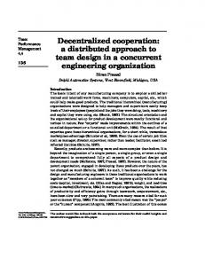
To meet the outlined requirements, an 8-tier data processing architecture has been elaborated, in which the lower levels are responsible for a stable and comprehensive world representation to be evaluated in the higher levels (figure 2). Layers 0 to 5 are processed locally in each node, while layer 6 contains the global processing activities. Layer 7 is again processed locally, but considering the results of inter-node correlation. In layer 0, the processing of the sensor input is performed, resulting in so-called modality or low-level symbols (LLS). Examples are "steps" in the audio and "person" in video modality. Each of these symbols is characterized with a number of properties like loudness or size in camera coordinates. Due to limited computing


resources of the embedded system for this layer, these symbols are afflicted by mistakes to a degree depending on environmental conditions. User Notification Filter

Layer 8

Detected alarms and unusual behaviour Predefined Alarm Recognition

Unusual Behaviour Recognition

Layer 7

Local and Neighbours Knowledge Layer 6 Inter-Node communication

Local Trajectories map Trajectories (e.g. Slope field)

Neighbour Node

Belief with and without evidence

Layer 5

HLS and associated instances Parameters inference

Layer 4

Semantic Processing Layers

Instances of high Level Symbols (HLS) Sensor fusion (audio, video)

Layer 3

Tracking-improved LLS instances at time t Tracking (t, t-1)

Layer 2

Plausibility checked LLS instances at time t

Global Processing Local Processing

Pre-processing of LLSs

Audio

Low Level Symbols ( S) Video

Layer 0

Low Level Layer

Figure 2: High Semantic Processing Layer Software Architecture Layer 1 tries to remove some of these by detecting outliers in the spatial domain (position, size). A set of templates is matched with the features detected in every frame. The templates are scaled in order to find objects of various sizes. In order to filter unrealistic primitives from the data stream, the average size of primitives is learned depending on their type and position in camera coordinates. The second plausibility check is in term of size and is done on bounding boxes to determine whether some person or object is blend into larger LLSs. In this case the count of smaller and larger primitives decides which kind of LLS is most probable and will be used for further processing. Symbols which pass the firsts spatial checks are submitted to a second check in layer 2. Their temporal behavior is checked, using a Markov Chain Monte Carlo based particle filtering approach to track the pre-processed symbols. The selected approach is particularly suited to track interacting objects. The output of this tier is a stable and comprehensive world representation including mono-modal symbols. Tier 3 is the sensor fusion tier, in which the mono-modal symbols are fused to form multi-modal symbols, also denoted as high-level symbols (HLS). Layer 4 is the parameter inference machine, in which probabilistic models for symbols’ parameters are optimized. The layer processes the incoming instances of fused primitive objects and adapts the parameters of the used probabilistic models to fit the data. The data are defined as the set of all the instances. The results of this tier are models of high-level symbols and features that describe object’s behavior. In tier 5, the system learns about trajectories of symbols, resulting in typical paths of instances in the space of the learned high level symbols through the view of the sensor node. They are represented by a learned transition matrix consisting of transition probabilities between model clusters. The matrix is learned by using a local search for the most likely sequence. Each HLS must therefore keep a list of all local trajectories to which the symbol belongs at the time t, in which an instance is being observed. The information gathered up to this layer is passed to the global processing unit in layer 6 to gain a global view of the system on the based of the local processing. In this layer, the communication to other nodes and the establishing of a global world view is performed. The trajectories are also used in this layer to find out, whether


a trajectory of one node can be extended to a neighboring node. In tier 7 the recognition of unusual behavior and events occurs with two approaches. One approach compares current high-level symbols with the learned models and trajectories. Therefore this module calculates probabilities for the 'existence' of symbols with respect to their position, velocity, direction, length of stay in a certain location, and probabilities for trajectories of symbols. It also calculates probabilities of the movement along trajectories, including trajectories across different nodes. Symbols with such probabilities below defined thresholds raise "unusual behavior" alarms. The second part of tier 7 is concerned with the recognition of pre-defined scenarios and the creation of alarms in case pre-defined conditions are met. Finally, layer 8 is responsible for communication to the user. It generates alarm or status messages and filters them, if particular conditions are announced too often or the same event is recognized by both methods in layer 7. 3

LOCAL PROCESSING UNIT

As just outlined, on a local level the input from each sensor is integrated in the node and used to progressively build-up a statistical description of the events sensed by that node. The observational data from the individual sensor modalities are provided as LLSs to the upper semantic levels. The LLSs are integrated into higher level semantic entities, HLSs, generated by an automatic clustering approach. The HLSs are events that occur repeatedly and generate characteristic patterns in the feature space, which are interpreted as learned normality. For instance, given the center of mass and speed of a detected person as input features, a possible typical pattern in this feature space is generated by persons taking repeatedly the same trajectory with approximately same velocity. Persons that sporadically take alternative routes will not affect the overall statistics but would be judged as unusual in layer 7. Finding main patterns in such feature space is the task of the local processing units. Thus, the patterns provide a description of the learned normality of object behavior. In the rest of the paper, we will use following convention for distinguishing between learned behavior or models and actually observed events. The learned models are denoted "HLS" for short, while the observed events are referred to as "HLS instances" or "instances" for short. The local processing unit is identified in figure 2 by layers 0 to 5. In the following sub-sections, we provide a specification of the feature selection and tracking procedure. Moreover, a definition of LLS and HLS is provided, which are respectively the low level features and the higher level semantic entities. Audio modality:

Video modality:

0.123.34 6.5 15 25 50 Y Y Y Y Y . . . Y

. .

Figure 3: example of instances of LLS 3.1 Features (LLS) The sensors are the low level processing units that provide to the upper semantic level the features used to learn objects behaviour in terms of LLSs. In the ongoing surveillance application we use both audio and visual input provided by a microphone array and a camera respectively. The audio objects are mainly used for detection of threats as predefined alarms. The used audio objects are the following: 1) scream; 2) breaking glass; 3) sound of walking; 4) shooting; 5) background noise and 6) not predefined. The visual LLSs provide to the upper semantic level the features needed for modality fusion, which generates instances of HLSs used to evaluate the object behavior. The visual LLSs considered are the following: 1) person; 2) person group; 3) luggage; 4) not classified object indoor and 5) not classified object outdoor. Regions corresponding to moving objects are extracted and a bounding box is associated to each region. For each detected region a set of properties to classify the object is computed, such as e.g. the position and size of


the bounding box, the percentage of pixels in the box belonging to foreground, the probability of correct classification. The list of attributes is fused between compatible modalities in the upper level and delivered to the next semantic level, in order to determine the properties of the HLS, as well as to compare to the learned HLSs in order to detect predefined or unusual behavior. In figure 3 are examples of instances of LLS for audio and video object. Note that some of the feature fields can be empty, depending on object modality. 3.2 LLS Tracking When having the first experimental results from the low-level feature extraction, it turned out that the detection is quite noisy. This has its origin in the performance of the embedded processors, on which the detection algorithms run. Due to the limited resources in spaces and power, the processors are also less powerful than standard desktop PCs for example. Therefore, it was decided to integrate an object tracking method in order to smooth the detection and make the results more a stable world representation. The tracking in this case is concerned with the problem of tracking multiple interacting targets. The objective is to obtain a record of the trajectories of targets over time and to maintain correct, unique identification of each target – otherwise applications like person tracking or others on the higher layers become impossible. Tracking multiple identical targets becomes challenging when the targets pass close to one another or merge as persons or other visual objects do in a crowd. Recent research in this direction overcomes the problem with the introduction of a motion model that is able to adequately describe target behavior also throughout interaction events [8]. The reason for using this motion model-based approach lies in the fact that the number of symbols in the observationk model (the world representation constructed from the low-level symbols) can change from sensor observation to sensor observation. E.g. if several persons are going through a corridor, the visual feature extraction algorithms might detect a satisfactory number of persons in one image and just a group of persons in the consecutive one. In case of unlucky conditions, the detection can change often within short periods of time for the same physical object. Additionally, the number of targets to be tracked can change every time, so the tracking method needs to be able to adapt to changing conditions in this respect. Normal particle filter-based tracking methods need the number of targets to be tracked as an input variable. Fortunately, there exists a mathematical trick to allow the above mentioned algorithm to cope with a varying number of interacting targets. This method minimizes the computational effort in comparison to joint particle filters for tracking of multiple targets and also minimizes the fault detection rate compared to a set of single-target-tracking particle filters. 3.2 Data Fusion and Parameter inference The LLSs corresponding to different modalities, audio and video, and to different object types, e.g. person and luggage, are merged according to pre-defined combination criteria in the succeeding layer. The fused LLSs are the HLS instances which are fed to the next layer for parameter inference. We use the data driven approach of [3] to learn normality. Clustering is achieved by using the Growing Neural Gas algorithm (GNG) [6]. The GNG provides an approximation of the data distribution that initially leads to an over-representation of the data in terms of representative vectors in the feature space, also called prototypes. At the same time, GNG establishes a topology of the prototypes. Subsequently, the prototypes are pruned in order to obtain a full covering of the data rather then a representation of the data distribution. The advantages of the approach are that the number of prototypes is automatically selected by the algorithm and the topology is also automatically generated. Moreover, even small clusters in the data distribution are located, as full data coverage is provided. However, the quality of the method is strongly affected by the precision of the underlying features. Clusters in the selected feature space provide a semantic model of the environment, else the HLSs. The prototypes are represented by Gaussian mixture models. The location of the center and the standard deviation of the distribution of the Gaussian mixture components provide a description of normality. The clusters define the semantic models of the environment. Additionally we learn the transition probabilities between neighboring semantic symbols. These are used to define paths of semantic symbols with a given probability to occur in the sensed area. The paths are determined by a local search procedure. 3.3 Semantic Models (HLSs) At the semantic inference level, HLS instances are analysed to produce High Level Symbols (HLSs), also called semantic symbols. HLSs represent learned behavior aspects. In our context, the HLSs are represented as bi-variate Gaussian distributions, also denoted as cluster. Therefore an HLS describes how the instances that belong to that cluster behave with respect to velocity, position, direction, power spectrum etc. Instances of LLSs are associated to the HLS with a certain probability. If the probability is below a threshold, the associated event is classified as unusual. Otherwise we say that the event is usual and the corresponding HLS is active at the


given time t. During the learning phase, which occurs at start-up of a node, the HLSs are established. Different sets of HLSs exist for the different LLS categories. Each HLS is specified by a set of features, as represented by the example in figure 4. The label is an index that describes the type of LLS. Other properties are the learned prior probability of activation of the HLS, the mean and variance of the standard distribution of attributes such as position, size, velocity and direction of arrival and loudness of sound. The “Power Spectrum Averaged” is given by the average values of the 16 frequency bands of the audio objects. The transition matrix describes the dynamics of the local environment. The matrix elements are the probabilities that an instance activating the HLS at time t is associated with another HLS at time t+1, under the constraint that the symbols are of the same type. The matrix is used to determine paths of HLSs. The weight matrix describes the global dependencies between symbols among different nodes, in terms of probability of co-activation of the symbols. The matrix is established in the succeeding layer, where inter-node communication occurs and is described in the following section, Sec. 4. As a matter of fact, even though the weight matrix is associated to each HLS, this uses multiple-nodes information, else non-local information. The entries in the weight matrix are learned in the phase of network establishment. However, we keep this information at the local level as this is associated to each HLS at learning phase. Semantic Model - HLS Label Probability Position (mean, variance) Size (mean, variance) Velocity (mean, variance) DirectionOfArrival(mean, variance) Loudness (mean, variance) PowerSpectrumAveraged TransitionMatrix WeightMatrix (see Sec.4 )

Figure 4: List of feature of the semantic model. Part of the features are represented by a bi-variate Gaussian distribution: f Label , k = N Label , k = N ( μ Label , k , Σ Label , k ) 4

ESTABILISHING THE NETWORK

The network is constituted by static sensors, each communicating with all the others via a wireless connection. The nodes do not have in the beginning any knowledge about their reciprocal neighborhood relationships. In particular, we assume that at least some of the nodes partly share a common sensing area. The task of network establishment consists in automatically learning the neighborhood relations between nodes, using at this scope the information provided at learning phase by the weights matrices, figure 5, describing the probability of co-activations of symbols between couple of nodes.

⎛ψ ij ( S li = 0, S mj = 0) ψ ij ( S li = 1, S mj = 0) ⎞ ⎜ ij i ⎟ ⎜ ψ ( S = 0, S j = 1) ψ ij ( S i = 1, S j = 1) ⎟ l m l m ⎝ ⎠ Figure 5: Elements of weight matrix between symbols l and m in nodes i and j The elements of the weight matrix in figure 5 are represented between symbols l and n in nodes i and j respectively. The status of the symbols is either active, S l = 1 , or not active, S l = 0 . Each entry in the matrix i

i

represents the probability of co-occurrence of the two possible states in the two symbols. In the previous section we describe the local learning phase, in which HLSs are set up on the base of a statistics of instances of HLSs. The local learning is followed by a global learning phase, in which in particular the neighborhood relationships are established. Information is exchanged among nodes, which is used to learn the probability of co-activation of HLSs as defined by the weight matrix in figure 5.


Ψ1112 ( S11 , S12 ) = Ψ1121 ( S12 , S11 ) Figure 6: Example of network establishment with two node and two HLSs per node The approach used for establishing the global knowledge is based on the fusion of two paradigms: 1) the loopy belief propagation algorithm [11][12] is used to share the information over the network and 2) a Boltzmann machine learning approach [1] is used as an update rule to learn the weigh matrix. The information exchange consists of an exchange of “beliefs” about the current state of the observed area. In the belief propagation approach, each node sends to all its neighbors a message that contains a probability, computed according to the information gathered by every neighbor, that the HLS of the receiver node is active or non active. This implies that the inference of local activation probabilities is supported not only by the local observations, but also from what neighbor nodes observe about the state of the receiver node. Messages from neighboring nodes are collected and used to update the belief of the receiver node. The belief is the probability that a given HLS in the node is active or not. It is computed using both local information and the messages received from neighbor nodes. The beliefs in each node are compared to the beliefs in neighboring nodes and in a Boltzmann learning fashion used for the computation of the elements of the weight matrix. The update rule of the weights follows the Boltzmann learning machine’s paradigm [1]. Figure 6 provides a visual representation of the described procedure of network establishment. Represented are the two sensors with overlapping sensing areas. This is schematically represented, in the bottom part of the figure 6, as two nodes, each containing two {1, 2}

HLSs. The first HLS in the two nodes, S1 , correspond to the overlap area of the two sensors (in green); the second ones correspond to the remaining part of the sensing area. The status of the symbols is active (1) or not {1, 2}

active (0). Correlations are learnt between the first symbols in the two nodes S1

S

, and the second symbols

{1, 2} , 1

represented in the figure 6 with a green link between the two symbols. Symbols 1 or 2 in the first node and 2, 1 in the second node respectively are not correlated. This is represented with the red link between the nodes. The links are symbolic representations of the corresponding elements of the compatibility matrix. 5

ALARM GENERATION

During the phase of network establishment, HLSs corresponding to different object types and relations between the HLSs are learned. HLSs are combined in a hierarchical way, in order to generate predefined scenarios, corresponding to events that we want to detect. Scenarios such e.g. unattended luggage, loitering persons etc. are described by such higher level symbols. Moreover, we also define an unusual behavior as a behavior that breaks the learned normality. This could be an instance that do not activate any of the learned symbols or that takes an unusual trajectory, which is defined as a temporal sequence of activations of HLSs. 5.1 Predefined Events This method takes the symbolic representation on the level of the modality related symbols as input. It uses a


rule-base to combine these symbols in a hierarchical way to create symbols with higher (more abstract) semantic meaning out of symbols with lower semantic level. Predefined alarms are not flexible and thus cannot adapt to new situations. Whatever is to be recognized has to be pre-programmed into the system before it becomes operative – as opposed to recognizing unusual behavior, which learns during operation. One advantage of recognizing predefined alarms is the ability to provide a human user with a semantic description of the type of alarm that the system has detected (e.g. “Unattended Luggage” instead of “Unusual Behavior”), also for complex scenarios. The other is that it can happen quite frequently that a specific type of mis-behavior is conducted – e.g. people walking in some wrong direction or in an area where it is not allowed – so the “unusuality” of such event decreases. With the pre-defined alarm feature such situations can be considered. 6

CONCLUSIONS AND OUTLOOK

We have presented a hierarchical processing architecture for a distributed sensor network, in which the single nodes are used to build up a semantic representation of the sensed environment which, shared with the neighbors by wireless communication, is used to create a common global representation. Step by step processing in each node is used to enrich the low level information with high level semantics. An innovative learning concept is presented in the way that communication between nodes is used to learn correlations among semantic symbols in different nodes. The system is used to learn usual events and pre-defined events that are used for threats detection in security surveillance. Future steps include extensive tests on real-life scenarios in an airport environment. REFERENCES [1] Ackley D. H., Hinton G. E., Sejnowski T.J., “A Learning Algorithm for Boltzmann Machines”, Cognitive Science, 147169, 1985. [2] Baker, C. R., Markovsky, Y., Greuen, J. van, Rabaey, J., Wawrzynek, J., and Wolisz, A. (2006), "Zuma: A plattform for smart-home environments", Proceedings of the 2nd IEEE International Conference on Intelligent Environments, 2006. [3] Bauer, D., Brandlem, N., Seer, S., Pflugfelder, R., (2006), “Finding Highly Frequented Paths in Video Sequences”, in Proc. ICPR 2006, 18th International Conference on Pattern Recognition, Volume 1, pp:387 - 391, 2006. [4] Crick C. and Pfeffer, A., (2003), “ Loopy belief propagation as a basis for communication in sensor networks”. In Proceedings of Uncertainty in Artificial Intelligence (UAI), 2003. [5] Foresti, G. L. , Regazzoni, C. S. , Varshney (eds.), P. K., " Multisensor Surveillance Systems: The Fusion Perspective", Kluver Academic Publishers, 2003, 978-1402074929 [6] Fritzke, B. (1995), “A Growing Neural Gas Network Learns Topologies”. In G. Tesaurso, D. Touretzky, and T. Leen, editors, Advances in Neural Information Processing Systems, pp 625–632. MIT Press, Cambridge, MA, 1995. [7] Herzner, W., Thuswald, M. (2001), "A Directory-Based Archive for Video Surveillance Systems", Proceedings of AVBS01 - 2nd European Workshop on Advanced Video-Based Surveillance Systems, Kingston upon Thames / UK, 4. Sep. 2001, pp.235-250. [8] Khan, Z., Balch, T., and Dellaert, F. (2006), “An MCMC-based Particle Filter for Tracking Multiple Interacting Targets”, IEEE Transactions on Pattern Analysis and Machine Intelligence, 2006. [9] Hochgatterer A, Prazak B, Russ G, Sallans B., "Behaviour Pattern Based Safety Assistant for the Elderly", in "Challenges for Assistive Technology", G. Eizmendi, J. Azkoitia, G. Craddock (Eds.), Proc. of 9th European Conference for the Advancement of Assistive Technology (AAATE'07), San Sebastian / SP, Oct. 3-5, 2007; IOS Press, (2007), ISBN: 978-158603-791-8; pp. 170-174 [10] Schimak, G, "Environmental Data Management and Monitoring System UWEDAT", Environmental Modelling & Software, Vol. 18 (2004), pp. 573-580 [11] Yedidia J. S., Freeman W. T., Weiss Y. (2000), “Generalized Belief Propagation”, MERL TR-2000-26, June 2000. [12] Yedidia J. S., Freeman W. T., Weiss Y (2002), “Understanding Belief Propagation and its Generalizations”, MERL TR2001-22, January 2002.