Wireless sensor networking has become an area of intense research activity. This is due to ... since they can patrol a wide area, and they can be re-positioned for better surveillance [7]. .... iterative multilateration [17]. This locationing ability is ...
A Distributed Self Spreading Algorithm for Mobile Wireless Sensor Networks Nojeong Heo and Pramod K. Varshney Department of Electrical Engineering and Computer Science, Syracuse University, Syracuse, NY 13244,USA {nheo,varshney}@syr.edu
Abstract - Sensor deployment is an important problem in mobile wireless sensor networks. This paper presents a distributed self deployment algorithm for mobile sensors. Performance metrics to evaluate algorithm performance are coverage, uniformity, time and distance traveled till the algorithm converges. Our algorithm is compared with a simulated annealing based algorithm for deployment and is shown to exhibit excellent performance.
1. Introduction Design and deployment of infrastructured networks such as a cellular network has matured over the last two decades. In such networks, mobile users access the network via fixed base stations. Planning and deployment of these networks is carried out based on radio propagation and terrain models with the goal of maximizing radio coverage. More recently, there has been a great deal of interest in ad hoc wireless networks. These networks employ fixed or mobile nodes and dynamically organize themselves into a network without requiring an infrastructure. In ad hoc networks, each node acts not only as an end node but also as a router. One important aspect in the design of these networks is the initialization procedure and establishment of routing structure. Most research on ad hoc networks has been focused on issues such as the development of routing protocols and quality of service and not on topology and deployment. Wireless sensor networking has become an area of intense research activity. This is due to technical advances in sensors, wireless communications and networking, and signal processing. Many applications are envisaged including environment monitoring, battlefield surveillance, and urban search and rescue especially in hazardous situations. Wireless sensor networks (WSN) operate under limited radio coverage and attempt to conserve bandwidth and battery power. Most of the research on WSN has focused on the development of collaborative signal processing and power aware algorithms [1]. Sensor nodes are generally assumed to be fixed and randomly placed because of practical reasons. The number of sensors is assumed to be quite large so that coverage of the surveillance area is not an issue. Not much attention has been paid to optimization in terms of number of nodes or their topology. Recently, Meguerdichian et al. have considered the problem of location and deployment of sensors in a WSN from a coverage standpoint [2]. They implicitly assumed fixed wireless sensor nodes. They argued that coverage is a primary performance metric that provides an indication regarding quality-of-service. They
combined computational geometry and graph theoretic approaches to develop algorithms for coverage calculations. We also focus on coverage in WSN and discuss it later in the paper. Bulusu et al.’s work [3] is somewhat similar to the deployment problem that is considered here. They have investigated the problem of adaptive beacon placement for localization in a WSN. They also pointed out the lack of viability and inadequacy of fixed and dense beacon placement in some situations due to node perturbation during deployment, noisy environment, and self-interference. By placing additional beacons incrementally, they achieve empirical adaptation to terrain conditions. Another related problem is the Art Gallery Problem in computational geometry [4]. The art gallery problem tries to find the minimal number of positions for guards or cameras so that every point in a gallery is observed by at least one guard or camera. A deterministic solution can be found for the art gallery problem and it appears to be a possible solution to a variety of sensor placement problems. Even though there are many solutions to the art gallery problem, all of them assume the availability of a good model of the environment a priori. However, it is virtually impossible to have complete information of the environment in a WSN. Too much communication over long range to obtain global information requires a huge amount of energy. This is an unaffordable burden on a system with limited power supply. Thus, deterministic deployment is impractical due to many reasons such as the harshness of deployment region that may be remote and inhospitable and the increased cost and latency due to the huge number of nodes deployed [5]. In our work, we are interested in the self-deployment of mobile sensor nodes. This is quite similar to problems considered in cooperative mobile robotics [6]. Mobile sensors are often desirable since they can patrol a wide area, and they can be re-positioned for better surveillance [7]. Some researchers considered the use of mobile robots in sensor networks. Winfield [8] considered autonomous dispersion of mobile nodes in a scenario where mobility is required to cover the entire region due to a lack of wireless network connectivity. He used a random diffusion method for node deployment while collecting data over a fixed surveillance region. In the incremental deployment algorithm [9], nodes are added one at a time. The goal is to maximize network coverage under the constraint that nodes maintain line-of-sight with each other. Loo et al. considered a system consisting of a number of cooperating mobile nodes that move toward a set of prioritized destinations under sensing and communication constraints [10]. They show how individual agents know when cooperation between agents improves the performance and when they should suspend cooperation.
Much research has been done about various issues related to the deployment problem. Most approaches use either a centralized solution as in the circle covering problem [11,12] and the geometric problem [13], or are restricted to a certain topology as in the coding theoretic approach [14]. Since some approaches adopt random deployment as in the set covering problem [5] and the topology discovery problem [15], initial distribution determines the utilization of networks. Our work is different from prior work on the deployment problem. Our deployment algorithm’s main objective is topology improvement for longer system lifetime by utilizing mobility of robots. We provide a decision and control mechanism at each robot to be used during deployment rather than random diffusion, which is used in Winfield’s work. In contrast to Howard et al. who use an incremental approach, the nodes in our algorithm are deployed at the same time and they organize themselves in an adaptive manner. Unlike Loo et al., our algorithm does not require prespecified destinations to form an energy efficient topology. Our self deployment algorithm will be more useful in situations where it is hard to ensure precise initial deployment due to the fact that the deployment area is too dangerous or inaccessible to humans. Randomly scattered sensors over a battlefield or a hazardous site are not likely to form a uniform distribution and provide desired coverage. Modification of WSN topology in an autonomous and distributed manner using our algorithm can help in improving sensor coverage and also to prolong expected system lifetime. This is essential in time-critical applications. For example, if some area is contaminated by a hazardous material, a properly deployed sensor network can quickly sense and measure the amount of hazardous material such as poisonous gas or nuclear leakage. By fully covering the entire area of interest, the overall condition can be assessed quickly and this information can be used for search and rescue missions as well as for evacuation route planning. The main goals of this paper are 1) discussion of the issue of coverage in WSN in detail 2) development of a distributed algorithm for self-deployment In the next section, we discuss performance metrics for a mobile WSN. In Section 3, we formulate the sensor deployment problem. Our algorithm is presented in Section 4 followed by simulation results in Section 5. Some concluding remarks are provided in Section 6.
2. Performance Metrics in Mobile WSN Selection of suitable measures to compare performances of different approaches is an important issue in a mobile WSN. Coverage, uniformity, time, and distance are considered as performance metrics in mobile wireless sensor networks here. Coverage and uniformity are related to the performance of sensor networks after the deployment of sensors is complete. Time and distance are directly related to the performance of the deployment scheme itself. Coverage Generally, coverage can be considered as the measure of quality of service of a sensor network. The concept of coverage as a paradigm for the system level functionality of multi-robot systems was introduced by Gage [16]. Gage described three types of coverage behavior for problems such as detection of targets over a surveillance area. These behaviors are: blanket coverage, where the objective is to obtain the maximum detection rate over a given
area; barrier coverage, where the objective is to minimize the probability of miss through the barrier; and sweep coverage, which is roughly equivalent to a moving barrier. Our self deployment algorithm can be classified as a blanket coverage problem according to Gage’s taxonomy. Coverage can be classified as either deterministic or stochastic by the manner in which nodes are deployed. To obtain deterministic coverage, sensor nodes should be placed at predefined locations. The art gallery problem is an example of deterministic coverage. By dispersing sensors randomly in the environment, stochastic coverage can be achieved. In this paper, coverage is defined by the ratio of the union of covered areas of each node and the complete area of interest. Here the covered area of each node is defined as the area within sensing radius R. Perfect detection of all interesting events in the covered area is assumed. C=
U Ai
i =1,..., N
A
where
Ai is the area covered by the ith node, N is the total number of nodes, A stands for the area of the region of interest(ROI).
If a node is located well inside the region of interest, the complete circle will lie within the ROI. In this case, the full area of that circle, i.e., πR 2 , is counted as the covered region. If a node is located near the boundary of the ROI, then only the partial area of the ROI covered by that node is included in the computation. Because of areas covered by nodes that fall out of the ROI and the fact that overlap of covered areas between nodes should not be included while computing coverage, we need to use more nodes than simply the ratio of A and area sensed by a single node. We distinguish sensing range and communication range of a node. In general, they will be different and accordingly sensing coverage and communication coverage will be different. Sensing coverage can be accrued when sensor nodes are connected via wireless links. Uniformity Uniformly distributed sensor nodes spend energy more evenly through the WSN than an irregular topology does. So, uniformity of network topology can be a good estimator for the expected system lifetime. Also, fewer nodes are required to cover an ROI when nodes are more evenly distributed. Uniformity can be defined by the average local standard deviation of the distances between nodes.
U=
1 N
Ui = ( where
N
∑U
i
i =1
1 Ki
Ki
1
∑ ( Di, j − M i )2 ) 2 j =1
N is the total number of nodes Ki is the number of neighbors of the ith node, Di,j is the distance between ith and jth nodes, Mi is the mean of internodal distances between the ith node and its neighbors.
In the calculation of the local uniformity Ui at the ith node, only neighboring nodes that reside within its communication range are considered. The uniformity measure is a local measure and is computed locally because each node has access to local information only. A smaller value of U means that nodes are more uniformly distributed in the ROI. In uniformly distributed networks, internodal distances are almost the same; the expected energy consumption per communication as well as the expected lifetime of each node is almost the same. Therefore, we can expect full energy utilization at each node and longer system lifetime for uniformly distributed networks.
Time The time spent for deployment is also important in many timecritical applications such as search and rescue and disaster recovery operations. Mostly, the required time depends on the complexity of the reasoning algorithm and physical time for the movement of nodes. The total time elapsed is defined here as the time elapsed until all the nodes reach their final locations. We focus here on the time spent for deployment itself and not on data transmission delays from a source node to a destination node that is commonly used for network performance evaluation and its quality of service. Distance The average distance traveled by each node is related to the required energy for its movement. So, the expected distance traveled is important for the estimation of required energy (fuel) when each node has a limited energy supply. The variance of traveled distance is also important to determine the fairness of the deployment algorithm and for system energy utilization.
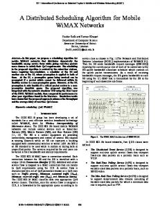
without any intervention from a central controller that acts remotely. We call this algorithm Distributed Self-Spreading Algorithm(DSSA) and discuss it in detail. To begin with, a specified number of nodes are pre-deployed randomly in a given region, for instance, inside a rectangle. The sensing range (sR) and the communication range (cR) are assumed to be given. Each node can sense or detect an event within its sensing range and any pair of nodes within their communication range can communicate with each other. This communication is needed for finding neighborhood, obtaining locations of nodes in the neighborhood, and transmitting and forwarding sensed data. Neighborhood is defined here as nodes within the communication range. The flow chart of the algorithm is given in Figure 1. This distributed algorithm is executed at each node i. Start Initialization p0, sR, cR Calculation of density µ,D0, D=D0
3. Mobile Node Placement/Deployment Problem
Calculation of partial force fni,j(µ,D,cR,pn)
3.1. Assumptions and restrictions
We assume that all sensor nodes have capabilities for sensing, communication, computation, and mobility. Sensing coverage and communication coverage of each node is assumed to be ideal, which means that both coverage areas have a circular shape without any irregularity. Computation capability is required at each node to support a distributed algorithm that includes a reasoning process for deployment and routing. We assume that the initial deployment is random and a distributed deployment algorithm will be executed starting from the initial random topology using each node’s mobility. Another assumption is that every node has the ability to know its own location by some method such as GPS or iterative multilateration [17]. This locationing ability is needed by each node while making a decision regarding its next movement in the deployment process. Also, we assume that there are no errors during transmissions of data and in the calculation of locations.
Temporary position pin+1' = pin + sum(fni,j)
Oscillation? |pin-1-pin+1'| < e
Covering and placement problem can occur in many applications from environment monitoring to battlefield surveillance. Without loss of generality, we can consider the covering problem in a rectangular ROI with a certain number of nodes that form an ad hoc wireless network. The goal is to find positions and movements of nodes to achieve maximum coverage and to form a uniformly distributed wireless network in minimum time and with minimum energy consumption. We develop a heuristic algorithm and evaluate its performance in terms of these performance metrics.
4. Distributed Self-Spreading Algorithm The algorithm is inspired by the equilibrium of molecules, which minimizes molecular electronic energy and inter-nuclear repulsion. Each particle obtains its own lowest energy point in a distributed manner and its spacing from the other particles is almost the same. While deploying a wireless sensor network using mobile nodes, we observe that a similar phenomenon is needed. We propose an algorithm that can cover the region of interest
Count oscillation Ocount = Ocount+1
No
pin+1=pin+1' Update D
Yes
Ocount < Olim No
No
Stable? |pin+1-pin| < e
pin+1=1/2(pin+pin+1') Update D
Yes
Count stable status Scount = Scount+1
The restriction is that each node has only local information from the neighboring nodes within its direct communication range. The communication range of each node is defined by the maximum distance at which the signal to noise ratio is above the threshold required for achieving the design goal in terms of power conservation.
3.2. Problem formulation
Yes
Scount < Slim Yes No
pin+1 = pin
Stop
Fig. 1 Distributed Self-Spreading Algorithm (DSSA) The algorithm begins with the specification of cR, sR, and the initial node locations (p0). In our algorithm, we require the quantity called expected density. This can be calculated by using
µ (cR) =
N ⋅ π ⋅ cR 2 , where N is the number of nodes and cR is the A
communication range of each node, and A is the ROI. Thus, expected density is the average number of nodes required to cover the entire area when these nodes are deployed uniformly. Initial local density D0 of a node is equal to the number of nodes within its communication range. These densities will be used when decisions regarding positions of nodes are made. We introduce the concept of force to define the movement of nodes during the deployment process. The force is dependent on the distance between nodes and the current local density. The force from a node that is closer is greater than that from a node that is farther just like the particles in Physics that follow Coulomb’s law.
We define a force function that satisfies the following conditions. (i) Inverse relation: f(d1) ≥ f(d2), when d1 £ d2 , where d1 and d2 are node separations from the origin. (ii) Upper limit: f(0+) = fmax. (iii) Lower limit: f(d) = 0, where d > dth, d is the node separation and dth is the threshold to define the local neighborhood. Condition (i) is the same as in Physics, but conditions (ii) and (iii) are included to modify the model to incorporate the notion of locality. In other words, a limiting function is applied via conditions (ii) and (iii). The partial force at time step n on the ith node from the jth node that is in the neighborhood of the ith node is calculated in this paper as
f ni , j = where
D
µ2
(cR − | p ni − p nj |)
p nj − p ni | p nj − p ni |
(1)
cR stands for communication range
p ni
stands for the location of ith node at time step n
The density factor, which is defined as the ratio of the local density (D) and the expected density (µ) at each node, is small in sparse regions and is large in dense regions. Also internodal distance affects the partial force inversely. Closely located nodes impose larger partial forces and nodes that are far apart induce smaller partial forces. After adding all the partial forces at the current location, each node can decide its next movement. The local information is collected from the nodes that are within the communication range and that information is used for the calculation of the local density at each node. Each node’s movement is decided by the combined force at that node due to nodes in its neighborhood. When should a node stop its movement is an important issue. Two stopping criteria are introduced in the Distributed SelfSpreading Algorithm. If a node moves less than e for the time duration Slim, this node can be considered to be in the stable status and that node stops its movement. This stopping criterion is for stationary nodes because of either empty fuel or broken mobile units and also for the nodes that have reached the stable status. If a node moves back and forth between almost the same locations many times, this node is regarded in the oscillation status. By comparing with the history of its movement, each node can know if oscillation is going on. Then one counts the number of oscillations and if this oscillation count (Ocount) is over the oscillation limit (Olim), we stop that node’s movement at the center of gravity of the oscillating points. When sensor nodes are deployed in a remote and hostile region, some nodes can be affected during and after deployment period. Some nodes can lose their mobility and other nodes can lose their communication functionality. So we need a robust deployment method that can handle these difficulties. Our algorithm exhibits this kind of robustness. First, when the sensor node loses its mobility, that sensor node does not move and is considered to be an early stopped node. Neighboring nodes, if they can move, may still improve the irregular topology. Second, when a sensor node loses its communication capability, that sensor node is of no use in a sensor network. Because each node’s movement is only affected by the current status of neighboring nodes, each node is adaptive to environment changes such as node failures, various terrain shapes, etc.
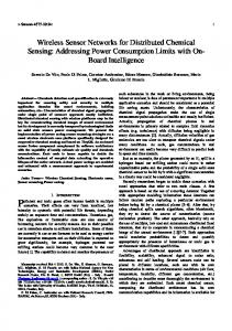
5. Simulation Results We consider 30 randomly placed nodes in a region of size 10 ¥ 10 to run the Distributed Self-Spreading Algorithm. We assume sR=2 and cR=4. Fig.2 shows the locations and coverage of the initial deployment before running the Distributed Self-Spreading Algorithm. Tiny circles represent the positions of nodes and small (shaded) and large circles are used to show the sensing range and the communication range respectively. Sensor information may be collected within the sensing range and communications between nodes are possible within the communication range. Communications are possible between nodes that are connected by a line in the figure. As seen in Fig 2., some parts of the region cannot be covered by the nodes that are randomly dispersed, even though there are enough numbers of them in the given ROI. In this particular example, the network is not fully connected, so the actual coverage is much smaller than just adding the entire covered region. The calculated coverage is more than 90%, but the actual coverage is well below 50% because the network is separated. This situation is exactly the case where topology improvement is required. Iintial position of 30 sensors, C = 0.93483 12
10
8
6
4
2
0
-2 -2
0
2
4
6
8
10
12
Fig. 2 Initial distribution of sensor nodes Fig. 3 shows nodes location and coverage after running the Distributed Self-Spreading Algorithm. The rectangle is fully covered after running the algorithm. The parameter values used in this simulation run are: stable status limit(Slim) =10, oscillation limit (Olim) = 10, and threshold (e) for oscillation and stable status =0.25994. Now the network is fully connected and also can cover the entire ROI. Note the spatial node distribution is more uniform than the initial random distribution in Fig. 2. Iteration # : 36, Covered Area: 1, Slim: 10, Olim: 10, e: 0.25994 12
10
8
6
4
2
0
-2 -2
0
2
4
6
8
10
12
Fig. 3 Final distribution after running DSSA
For the purpose of comparison, Simulated Annealing was also used for self-spreading. Simulated Annealing algorithm is known as a good solution of many combinatorial optimization problems. To implement a Simulated Annealing algorithm, 4 main design issues should be considered. These are: the definition of the neighborhood, move operator, local energy calculation, and annealing schedule. The definition of neighborhood is the same as for DSSA, i.e., it is set equal to the communication range. This concept of neighborhood is reasonable because each node can only reach the neighboring node in a single hop communication. The move operator is chosen to be a random movement within the neighborhood. The local energy calculation is done by adding up sub-forces in the neighborhood just like our algorithm. The exponential cooling schedule is used as the annealing schedule for efficiency as in [18]. The parameters used are initial temperature T0=1 and as the stopping criterion 3 consecutive failure of achieving the desired acceptance ratio is used. The result after applying the simulated annealing algorithm is shown in Fig. 4. Fig. 4 shows that Simulated Annealing also works well for this initial distribution. The entire area is covered by 30 sensor nodes and these nodes are well spread over the region. Iteration # : 19, Covered Area: 1, T0: 1, failureIndexLimit: 3 12
10
8
6
InitstdSeparation, stdSeparation 1.6 1.4 1.2 1 0.8 0.6 0.4
Initial SA
0.2 0 10
Our 15
20
25
30 # of Nodes
35
40
45
50
Fig. 6 Uniformity versus network size Fig. 5 shows the improvement in coverage area from the initial random deployment for both algorithms; simulated annealing and ours. Though both algorithms have quite similar performance, our algorithm has better coverage for smaller number of nodes. As the number of nodes increases, the improvement in coverage diminishes. Standard deviation of internodal distances can be considered as the metric of uniformity of the networks. Fig. 6 shows the reduction in the standard deviation from the initial case. Both algorithms obtain better uniformity than the initial one and ours outperforms simulated annealing. The improvement in uniformity is not that different with varying network density.
4
stoppedNum 35
2
30 0
25 -2 -2
0
2
4
6
8
10
12
20
Fig. 4 Final distribution after running SA
SA
15
The performance of our algorithm is evaluated in terms of the metrics presented in Section 2. Results are presented in Fig. 5 ~ 8. These results are obtained for different number of nodes dispersed over a fixed ROI of size 10 ¥ 10, i.e., for different node densities. Number of nodes varies from 10 to 50 and results are averaged over 100 runs.
Our 10
5
0 10
15
20
25
30 # of Nodes
35
40
45
50
Fig. 7 Termination times versus network size InitArea & Covered Area 1 meanTotalDistance
Our 0.95
80
SA 70
0.9
60 50
Initial Area
0.85
SA
40 0.8 30 0.75
20 10
0.7 10
15
20
25
30 # of Nodes
35
40
45
Fig. 5 Coverage versus network size
Our
50 0 10
15
20
25
30 # of Nodes
35
40
45
50
Fig. 8 Distance traveled versus network size
Fig. 7 shows that our algorithm leads to faster deployment than simulated annealing. Also termination times of our algorithm are similar over a wide range of number of nodes. This means that our algorithm is more insensitive to the number of nodes, i.e., network density. Fig. 8 shows mean distance traveled to reach the final locations for deployment. Our algorithm requires less distance traveled than the simulated annealing algorithm. This distance is related to the required energy (fuel) for deployment. Also, we observe that the required energy as well as the distance traveled at different node densities is almost constant. Thus, the required energy (fuel) is quite insensitive to network density. As seen in Fig.5~Fig.8, 25~40 nodes are required to attain acceptable performance. When too few nodes are used, we cannot obtain full coverage over the region of interest. When too many nodes are used, we do not gain that much coverage improvement because of the diminishing marginal gain in terms of coverage, though we can still obtain more uniform distribution. With the number of nodes in this range, the required time and distance of our algorithm is much smaller than that of the Simulated Annealing algorithm. Because the variation of required time and traveled distance is small over this range of node densities, it is easy to estimate the required energy for deployment.
6. Conclusions We considered the sensor coverage problem for the deployment of wireless sensor networks here. A region of interest needs to be covered by a given number of nodes with limited sensing and communication range. We start with a “random” distribution of the nodes over the region of interest. Though many scenarios adopt random deployment because of practical reasons such as deployment cost and time, random deployment may not provide a uniform distribution which is desirable for a longer system lifetime over the region of interest. In this paper, we propose a distributed algorithm for the deployment of mobile nodes to improve an irregular initial deployment of nodes. After going through the algorithm, the area of interest is covered by uniformly distributed nodes. While developing the algorithm, one should consider factors such as density of nodes, memory constraints, localization errors, and scalability of mobile nodes. Through the requirement of mobility and locationing ability of nodes, this algorithm provides a way to avoid expensive redeployment process. This postdeployment idea will be more useful especially when a large fraction of nodes are destroyed or broken during deployment or in a hostile situation, where initial distribution is quite uneven and when redeployment is too costly or too risky. The performance of the algorithm is determined by the percentage of region covered, by computational/deployment time, by the mean distance that is required for the deployment, and by the uniformity of the networks. Simulation results show that our algorithm successfully obtains a uniform distribution from initial uneven distribution. The performance of our algorithm is compared with the Simulated Annealing algorithm and exhibits excellent performance.
Acknowledgments This work was supported in part by the National Science Foundation under grant number ECS-9901361 and by NASA under grant number NAG5-11227.
References [1] Kumar, S.; Feng Zhao; Shepherd, D., “Collaborative signal and information processing in microsensor networks,” IEEE Signal Processing Magazine, vol.19, no. 2, pp. 13 -14, Mar. 2002.
[2] Seapahn Meguerdichian, Farinaz Koushanfar, Miodrag Potkonjak, and Mani Srivastava, “Coverage Problems in Wireless Ad-hoc Sensor Networks,” IEEE Infocom, pp. 1380-1387, 2001. [3] Nirupama Bulusu, John Heidemann, and Deborah Estrin, “Adaptive Beacon Placement,” in Proceedings of the 21st International Conference on Distributed Computing Systems, pp. 489-498, Phoenix, AZ, Apr. 2001. [4] O'Rourke, J., Art Gallery Theorem and Algorithms. New York: Oxford University Press, 1987. [5] S. Slijepcevic and M. Potkonjak, “Power efficient organization of wireless sensor networks,” Proceedings of IEEE International Conference on Communications, 2001. [6] Cao, Y. U., Fukunaga, A., and Kahng, A., “Cooperative mobile robotics: Antecedents and directions,” Autonomous Robots, vol. 4, pp. 1–23, 1997. [7] H. Qi, S. S. Iyengar and K. Chakrabarty, “Distributed sensor fusiona review of recent research”, Journal of the Franklin Institute, vol. 338, pp. 655-668, 2001. [8] A.F.T. Winfield, “Distributed sensing and data collection via broken ad hoc wireless connected networks of mobile robots,” in Distributed Autonomous Robotic Systems 4, eds. LE Parker, G Bekey & J Barhen, Springer-Verlag, pp. 273-282, 2000. [9] Andrew Howard, Maja J Mataric´ and Gaurav S. Sukhatme, “An Incremental Self-Deployment Algorithm for Mobile Sensor Networks,” To appear in Autonomous Robots Special Issue on Intelligent Embedded Systems, 2002. [10] Lit-Hsin Loo, Erwei Lin, Moshe Kam and Pramod Varshney, “Cooperative Multi-Agent Constellation Formation under Sensing and Communication Constraints,” in Cooperative Control and Optimization, pp.143-170, Kluwer Academic Press, 2002. [11] J. B. M. Melissen, P. C. Schuur, “Improved coverings of a square with six and eight equal circles,” Electronic Journal of Combinatorics, vol.3, no.1, 1996. [12] K. J. Nurmela, P. R. J. Östergård, “Covering a square with up to 30 equal circles,” Research Report A62, Laboratory for Theoretical Computer Science, Helsinki University of Technology, 2000. [13] K. Sugihara and I. Suzuki, “Distributed Algorithms for Formation of Geometric Patterns with Many Mobile Robots,” Journal of Robotic Systems, vol.13, no.3, pp. 127-139, 1996. [14] K.Chakrabarty, S.S.Iyengar, H.Qi, E.Cho, “Coding theory framework for target location in distributed sensor networks,” IEEE International Conference on Information Technology: Coding and Computing, June 2001. [15] Roger Wattenhofer, Li Li, Paramvir Bahl, Yi-Min Wang, “Distributed Topology Control for Wireless Multihop Ad-hoc Networks,” Proceedings IEEE INFOCOM 2001, pp. 1388-1397, 2001. [16] Gage, D. W., “Command Control for Many-Robot Systems,” AUVS-92, the Nineteenth Annual AUVS Technical Symposium, Huntsville AL,22-24 June 1992. Reprinted in Unmanned Systems Magazine, Vol. 10, No. 4, pp 28-34, Fall 1992. [17] K. Sohrabi, B. Manriquez, and G. Pottie, “Near-ground wideband channel measurements,” In Proceedings of the 49th Vehicular Technology Conference (Houston, May 16–20), IEEE, New York, 1999, pp. 571–574. [18] S. Kirkpatrick, C.D. Gelatt, and M.P. Vecchi, “Optimization by simulated annealing,” Science, vol. 220, pp. 671-680, 1983.