Distributed Adaptation Methods for Wireless Sensor

Department of Computer Science

Publications Southern Illinois University Carbondale

Year 

Distributed Adaptation Methods for Wireless Sensor Networks R. R. Brooks∗

M. Pirretti†

Mengxia Zhu‡

S. S. Iyengar∗∗

∗ Pennsylvania

State University State University ‡ Louisiana State University and Agricultural & Mechanical College, [email protected] ∗∗ Louisiana State University and Agricultural & Mechanical College Published in Brooks, R. R., Pirretti, M., Zhu, M., Iyengar, M. (2003). Distributed adaptation methods for wireless sensor networks. IEEE Global Telecommunications Conference, 2003. GLOBECOM ’03, vol.5, 2967 - 2971. doi: 10.1109/GLOCOM.2003.1258778 2003 IEEE. Personal use of this material is permitted. However, permission to reprint/republish this material for advertising or promotional purposes or for creating new collective works for resale or redistribution to servers or lists, or to reuse any copyrighted component of this work in other works must be obtained from the IEEE. This material is presented to ensure timely dissemination of scholarly and technical work. Copyright and all rights therein are retained by authors or by other copyright holders. All persons copying this information are expected to adhere to the terms and constraints invoked by each author’s copyright. In most cases, these works may not be reposted without the explicit permission of the copyright holder. † Pennsylvania

This paper is posted at OpenSIUC. http://opensiuc.lib.siu.edu/cs pubs/4

Distributed Adaptation Methods for Wireless Sensor Networks R.R Brooks, M. Pirretti Penn State Applied Research Laboratory

M. Zhu, S. S. Iyengar Department of Computer Science Louisiana State University

Abstract- This paper presents distributed adaptation techniques for use in wireless sensor networks. As an example application, we consider data routing by a sensor network in an urban terrain. The adaptation methods are based on ideas from physics, biology, and chemistry. All approaches are emergent behaviors in that: (i) perform global adaptation using only locally available information, (ii) have strong stochastic components, and (iii) use both positive and negative feedback to steer themselves. We analyze the approaches’ ability to adapt, robustness to internal errors, and power consumption. Comparisons to standard wireless communications techniques are given. Keywords: Sensor networks, adaptation, emergence I. INTRODUCTION In this paper we present four distributed adaptation methods for use by wireless sensor networks (WSNs) in Military Operations in Urban Terrain (MOUT) scenarios. Urban scenarios are challenging since obstructions to radio communications may cause the shortest path between two points to not be a straight line. The chaotic nature of MOUT missions means paths are not reliable. Only transient paths may exist. In spite of this, timely communications are required. Our approaches use local decisions to adapt to a constantly changing substrate. The insights we gained by testing these adaptation methods are being used to design and implement wireless routing protocols. The four methods we analyze are: (i) Spin Glass, (ii) Multifractal, (iii) Coulombic, and (iv) Pheromone. A. Wireless Sensor Network (WSN) Definition A WSN is a set of sensor nodes monitoring their environment and providing users with timely data describing the region under observation. Nodes have wireless communications. Centralized control of this type of network is undesirable and unrealistic due to reliability, survivability, and bandwidth considerations [1]. Distributed control also has other advantages: i) increased stability by avoiding single points of failure, ii) simple node behaviors replace complicated global behaviors, and iii) enhanced responsiveness to changing conditions since nodes react immediately to topological changes instead of waiting on central command. Our definition of a WSN does not preclude nodes being mobile. B) WSN Applications Consider the WSN application in [2], a surveillance network tracks multiple vehicles using a network of acoustic, seismic and infrared sensors. For a MOUT application, it is essential that the user community have timely track information. Figure 1 shows an idealized MOUT terrain. Walls are objects which block radio signals, such as buildings. Open cells are open regions allowing signal transmission. Open doors (closed doors)

GLOBECOM 2003

are choke points for signals that are open (closed). Finally, obstructions are intermittent disturbances that occur at random throughout the sensor field. Random factors are inserted to emulate common disruptions for this genre of network. Each square capable of transmission contains a sensor node. This amounts to having a sensor field with a uniform density. This provides an abstract example scenario approximating situations likely to exist in a real MOUT situation. This allows us to examine multiple adaptation techniques without being distracted by implementation details. After evaluating adaptation at this abstract level, the insights gained can then be used to create more robust routing protocols.

Figure 1. Idealized urban terrain. C) WSN Requirements WSN applications will typically require a large number of nodes to adequately determine the number, position, and trajectories of the objects under observation. To be affordable, individual nodes will be inexpensive and thus unreliable. Power consumption is an important issue. Our goal is to design a WSN that is fault tolerant, consumes minimal resources, supports secure message passing, and adapts well to environmental changes. II. SPIN GLASS The Spin Glass method uses the Ising model. Locally interacting magnets generate a macroscopic magnetic field. Field intensity depends on a kinetic factor. No macroscopic field exists when randomly pointing magnets cancel each other out. Magnets can align in metals like iron creating a perceptible magnetic field. We apply a similar concept to route data in an ad hoc sensor network. Our simulations use a two-dimensional MOUT scenario like figure 1. Each cell is a miniature magnet pointing in one of eight cardinal directions as its next hop on its way to the data sink. A potential energy field is established by data propagat-

- 2967 -

0-7803-7974-8/03/$17.00 © 2003 IEEE

Authorized licensed use limited to: Southern Illinois University Carbondale. Downloaded on March 18,2010 at 11:18:28 EDT from IEEE Xplore. Restrictions apply.

ing hop by hop from the data sink, defining the minimum number of hops from each node to the data sink. One or more sink(s) can exist. Cells attempt to find optimal routes to the nearest data sink. Link failures update the potential field locally. This change diffuses through the system starting where the error occurs. Some disturbances are minor (ex. no other nodes depend on the link, or equally good alternatives exist). If a link serves is a critical routing point, minor errors can cause phase changes in the system. The node’s spin direction (data route) is a combination of the potential field and a kinetic factor. It follows the Boltzmann distribution: P[s] = e-E(s) / KT / ΣAe-E(A) / KT

Spin Glass Comm unication Cost 6000

4000 3000 2000 1000 0 1

5

9

13

17

21 25 29

33

37

41 45 49

53

57

Generation#

Fig. 3. Spin Glass Communication Cost III. MULTI-FRACTAL Witten and Sander introduced the multi-fractal crystal-growing model in the early 1980s. On contact with foreign seeds, gas or fluid particles begin to solidify when crystallization conditions are satisfied. Crystal growth is inhibited by nearby particles due to interfacial surface tension and latent heat diffusion.

Low T High T Disturb

Spin Glass Mean Distance 300

W/ O Dist ur bance Wit h Dist urbance

5000

(1)

Instead of enumerating all possible configurations in the denominator,, only eight possible local configurations (the cardinal directions) are used. This reduces the computation needed and also removes the need for global information.

250 200 150

Multi-fractal Mean Distances 300

100

Mean Distance

Mean Distance

nications overhead. To quantify the amount of energy consumed we compute the total number of messages sent and their size. Fig. 3 shows communications cost with and without two topological disturbances.

50 0 1

4

7 10 13 16 19 2

2

2 31 3

3

4

4

4

4

5

5

5 61

250 200 150 100

W/O Disturbance

50

With Disturbance

0

Generation#

1

4

7 10 13 16 19 22 25 28 31 34 37 40 43 46 49 52 55 58 61

Generation#

Fig. 2. Spin Glass Mean Distance If a cell points to neighbor s, E(s) represents s’s potential value minus the cell’s potential value. K is the Boltzmann Constant and T is temperature. When T is large cells have an equal probability of pointing in any direction, regardless of their neighbors’ potential energy. When T is small, cells are more likely to point towards low energy neighbors. If T is at or below the freezing point, the system is in a rigid state and does not respond to its environment. T is important, because the shortest path is not the only important factor. A large T may reduce the power drain on choke points by data taking longer routes. A low T can protect the system by reducing oscillations in the system. T can be specified on a per-region basis, allowing flexible control of the system. To quantify system adaptation we measure the average distance from each node to the data sink. Fig. 2 shows the mean number of hops versus generation number (time step) for a low temperature system (Low T), high temperature system (High T), and a system with a topological disturbance (Disturb). Topological disturbances correspond to choke points in figure 1 opening or closing. The system converges well when T is small, but not when T is large. Topological disturbances are accommodated after a number of fluctuating generations. Figure 3 shows system power consumption. This is indicative of system scalability. Our analysis considers only commu-

GLOBECOM 2003

Fig. 4. Multi-fractal Mean Distance In Multi-fractal routing, the data sink is the foreign seed. A routing tree grows from the seed. The tree is essentially a space-filling curve. Based on the number of neighboring tree nodes, a set of probabilities for joining the routing tree were derived. Cells are less likely to join the tree as the number of neighboring tree cells increase, similar to crystallization inhibition. The probabilities define the growth rate and structure of the routing tree. When topological disturbances occur, link failures propagate down the tree removing invalid routing table entries. Fig. 4 shows the mean number of hops per generation number (time step) with and without topological disturbances (as for the Spin Glass model in fig 2.). Fig. 5 shows power consumption with and without a disturbance. Multi-fractal Communication Cost 600 W/O Disturbanc e

500

With Disturbanc e

400 300 200 100 0 1

5

9

13

17

21 25

29 33 37

41 45 49 53 57

Generation#

Fig. 5. Multi-fractal Communication Cost

- 2968 -

0-7803-7974-8/03/$17.00 © 2003 IEEE


Charge Diminish Rate Vs. Communication Events (out of 128256 possible events)

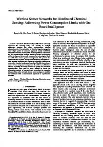
IV. COULOMBIC MODEL The Coulombic model is a preprocessing step for use with the pheromone approach discussed in section V. The goal is for data sources to be evenly distributed throughout the network. Data packets find the data source nearest to their node. Pheromone routing is then used to maintain efficient routes between data sources and sinks. A similar approach applied to sensor node placement for sensing coverage is in [3]. The Coulombic model is roughly based on charged particle interactions defined by Coulomb’s Law: (2)

where F is the amount of force on each particle, q1 is the net charge on particle 1, q2 is the net charge on particle 2, ε0 is the constant permittivity of free space, and d is the distance between the particles. We utilize two properties of Coulomb’s Law: (i) the relationship between distance and force and (ii) the interactions between the particles are all independent. This allows the approach to rely solely on local information and peer-to-peer interactions. Node Count Vs Mean Distance for Multiple Parameter Sets Mean Distance of Freecells from Closest Datasource

9 8 7 6 5 4 3 2 1 0 0

10

20

30

Node Count

40

DR =.1 TR = .1 DR = .1 TR =.3 DR = .1 TR = .5 DR = .1 TR = .7 DR = .1 TR = .9 DR = .3 TR = .1 DR = .3 TR = .3 DR = .3 TR = .5 DR = .3 TR = .7 DR = .5 TR = .1 DR = .5 TR = .3 DR = .5 TR = .5 DR = .7 TR = .1 DR = .7 TR = .3 DR = .7 TR = .5 DR = .9 TR = .1 50 DR = .9 TR = .3 DR = .9 TR = .5

Fig. 6. Performance for various parameters Data sources are particles with equal charge and polarity. The sensor nodes are called free cells, act as vessels through which force can be transmitted. Since we are attempting to evenly distribute data sources only one polarity is needed. The global behavior of having well distributed data sources emerges from the local node behaviors. Data sources transmit force to their neighbors. The neighboring nodes in turn transmit a percentage of their force to their neighbors, etc. In essence this approximates the inverse exponential relationship between the forces on particles and the distance between them. The system has no memory, allowing the peer-to-peer behaviors to rely solely on local information.

GLOBECOM 2003

Communication Events

104891

100000 80000 60000

55910

40000 28270 20000

14443

7604

0 0

0.03

0.06

0.09

0.12

0.15

0.18

0.21

0.24

Charge Diminish Rate

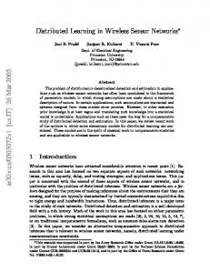
Fig. 7. Parameter effect upon power For the Coulombic model, we measure the mean distance of “free cells” from their closest data source. Fig. 6 shows this for various parameter sets. The DR (TR) parameter controls how rapidly forces dissipate (diffuse) in the system for each generation of the algorithm. Parameter settings with squares (triangles and x’s) are optimal (suboptimal). Charge Dim inish Rate Vs. Mean Distance of Freecells to Nearest Datasource 3.5

Mean Distance of Freecells to Nearest Datasource

F = q1*q2 / (4π ε 0d2),

121635

120000

3

2.5 2

1.5 1

0.5 0 0

0.02

0.04

0.06

0.08

0.1

0.12

0.14

0.16

0.18

0.2

0.22

0.24

Charge Dim inish Rate

Fig. 8. Parameter effect upon performance To tune the time needed for the Coulombic model to converge to a steady state, the charge diminish rate parameter was introduced. The charge associated with each data source decreases over time. Steady state occurrence can be predicted using the following equation: N = ln(Ts) / -CDR,

(3)

where N is the number of generations through the model, Ts is the Stopping Threshold parameter, and CDR is the Charge Diminish Rate parameter. The charge diminish rate parameter has direct control over how rapidly the quantity of messages being sent approaches a steady state behavior. Fig. 7 shows how the relationship between power consumption and the charge diminish rate parameter. Fig. 8 shows how varying this parameter affects the data source distribution. Note that a charge diminish rate of around 0.04 has good performance and low power consumption. V. PHEROMONE The pheromone model used is based on how ants forage for food and related to the approach in [4]. Data sources (sinks) are ant nests (food). Messages are ants. Ants attempt to find

- 2969 -

0-7803-7974-8/03/$17.00 © 2003 IEEE


paths between the nests and food sources. They release two different pheromones: (i) search pheromone when they look for food and (ii) return pheromone when they have food and return to the nest. The ants also follow a random walk, but they also search for the opposite pheromone of the one they currently release. Ants searching for food tend to follow the highest concentration of return pheromone. Ants returning to the nest tend to follow the highest concentration of search pheromone. This is modeled as a probability distribution where each ant is more likely to move following the pheromone gradient. The approach in [4] was designed for wired networks. Our scenario is more similar to an open field. In our initial implementation a pathology was noticed where ants moving two and from the data sink would form a cycle. To counteract this, we caused the ants to be repulsed by the pheromone they currently emit. A parameter was created denoting the relative strength of repulsion and attraction. This compels ants not to stay in one area and solved the pathology. To evaluate this algorithm we measure the number of hops an ant needs to make a round trip from its nest to a food source. Fig. 9 plots this versus the repulsion ratio. A ratio of approximately 80% works best. Optim al Repulsion Ratio 255

Average Path Length

250 245 240 235 230 225 220 215 210 0.2

0.4

0.6

0.8

0.9

1

1.2

1.4

1.8

2.5

5

Repulsion Ratio

Fig. 9. Effect of repulsion on performance VI. PROTOCOL COMPARISON AND DISCUSSION Many routing protocols have been proposed for WSNs. The Link State (LS) routing algorithm requires global knowledge about the network. Global routing protocols suffer serious scalability problem as network size increases [6]. DestinationSequenced Distance-Vector algorithm (DSDV) is an iterative, table-driven, and distributed routing scheme that stores the next hop and number of hops for each reachable node. The routing table storage requirement and periodic broadcasting are the two main drawbacks to this protocol.[6] In Dynamic Source Routing Protocol (DSR), a complete record of traversed cells is required to be carried by each data packet. Although no up to date routing information is maintained in the intermediate nodes’ routing table, the complete cell record carried by each packet imposes storage and bandwidth problems. Ad-Hoc On Demand Distance Vector Routing Algorithm (AODV) alleviates the overhead problem in DSR by dynamically establishing route table entries at intermediate nodes, but symmetric links are required by AODV. Cluster-head Gateway Switch Routing (CGSR) use DSDV as the underlying routing scheme to hierarchically address the network. Cluster head and

GLOBECOM 2003

gateway cells are subject to higher communication and computation burden and their failure can greatly deteriorate our system [5]. Greedy Perimeter Stateless routing algorithm (GPSR) claims to be highly efficient in table storage and communication overhead. However, it heavily relies on the self-describing geographic position, which may not be available under most conditions. In addition, the greedy forwarding mechanism may prohibit a valid path to be discovered if some detouring is necessary [7]. The Spin Glass and Multi-fractal models are related to the table-driven routing protocols by establishing routes from every cell to data sink(s). These protocols ensure timely data transmission on demand without searching for the route each time. The Ant Pheromone model is related to the packet-driven protocols. Ants can be viewed as packets traversing from data sources to data sinks. All of the models we presented are decentralized, using only local knowledge at each node. They dynamically adapt to topological disturbances (path loss). Storage requirements for the routing table of Spin Glass and Multi-fractal are low compared with most other protocols, while the Ant Pheromone’s storage requirements are even lower than these two. The Temporally Ordered Routing Algorithm (TORA) is a source initiated and distributed routing scheme that shares some properties with the Spin Glass model. It establishes an acyclic graph using height metric relative to the data sink and also has local reaction to topological disturbances [5]. The kinetic factor in our Spin Glass model and the frequency of ant generation in the Ant Pheromone model provides the system with flexibility in controlling routing behaviors under various conditions. Route maintenance overhead is moderately high for the Spin Glass model. The Multi-fractal approach, as a probabilistic space-filling curve, has very light computation and communication load, and overhead is saved in route discovery and maintenance. This is at the cost of a higher distance to the data sink(s). Route maintenance overhead for the pheromones is low due to the reduced number of nodes involved in each path. Since the Multi-fractal model strives to cover the sensor field by using as few cells as possible, the sparse routing tree sparse conserves energy. The shortest routes to the data sink are not found using the Multi-fractal model. On the other hand, Spin Glass model is more sensitive to internal errors since any possible error may diffuse throughout the network. The Multi-fractal and Ant Pheromone models are very resistant to internal errors. The time required for the Ant Pheromone algorithm to converge to a steady state is much longer than required by the other two adaptations. For applications requiring short data paths, the Spin Glass model is preferred. For overhead sensitive applications that require quick deployment, the Multi-fractal model is a better candidate. If error resilience and low overhead are the principle requirements, then the Ant Pheromone model is appropriate. Hybrid methods or switching between methods at different phases may be useful.

- 2970 -

0-7803-7974-8/03/$17.00 © 2003 IEEE


VII. CONCLUSION The purpose of our work is to develop adaptive networking methods for ad hoc WSNs. We performed analyzed the algorithms based on resource consumption, fault tolerance, number of nodes required, sensitivity to algorithm parameters, and critical points where phase changes occur. This conference paper summarized some of our results. We are now using these insights to design wireless routing protocols in conjunction with researchers at the University of Wisconsin. Two applications are foreseen for these adaptive protocols. One application is for the system to tolerate intermittent hibernation by a non-negligible subset of the WSN nodes. This should significantly prolong the lifetime of the system. The other application is to maintain multiple routes to a single data sink. This should both prolong the system lifetime and support information assurance requirements. In addition to this, we are continuing our analysis of system adaptation. A unifying abstraction is being considered that contains these approaches as a subset. It may then be possible to analytically derive local behaviors to maintain globally desirable system attributes. Our approach is to consider and test the adaptation problems of the system at an abstract level first. Insights gained at this level can then be used in protocol design and implementation. We are currently designing the protocols for implementation and testing with standard network tools like NS-2.

REFERENCES K. Chang, C. Chonge, and Y. Bar-Shalom, “Joint Probabilistic Data Association in Distributed Sensor Networks,” IEEE Transactions on Automatic Control, vol. AC-31, pp. 889-897, 1986. [2] R. R. Brooks, P. Ramanathan, and A. Sayeed, “Distributed Target Tracking and Classification in Sensor Networks,” Proceedings of the IEEE, Invited Paper, Accepted for Publication, February 2003. [3] Y. Zou and K. Chakrabarty, “Sensor Deployment and Target Localization Based on Virtual Forces.” IEEE Infocom Conference, 2003. [4] Marco Dorigo, Vittorio Maniezzo, Alberto Colorni, “The Ant System: Optimization by a colony of cooperating agents,” IEEE Transactions on Systems, Man, and Cybernetics Part B. 26(1):29-41, 1996 [5] Elizabeth M. Royer. A Review of Current Routing Protocols for Ad Hoc Mobile Wireless Networks IEEE Personal Communication April 1999 [6] James F. Kurose and Keith W. Ross Computer Networking a Top-Down Approach Featureing the Internet AW Higher Education Group 2003 [7] Brad Karp and H.T.K Ung Greedy Perimeter Stateless Routing for Wireless Networks Proc. of the 6th Annual ACM/IEEE International Conference on Mobile Computing and Networking 2000

[1]

Acknowledgement and disclaimer: This research is sponsored by the Defense Advance Research Projects Agency (DARPA), and administered by the Army Research Office under Emergent Surveillance Plexus MURI Award No. DAAD19-01-10504. Any opinions, findings, and conclusions or recommendations expressed in this publication are those of the authors and do not necessarily reflect the views of the sponsoring agencies.

GLOBECOM 2003

- 2971 -

0-7803-7974-8/03/$17.00 © 2003 IEEE
