A PARALLEL ROBIN-ROBIN DOMAIN DECOMPOSITION METHOD

A PARALLEL ROBIN-ROBIN DOMAIN DECOMPOSITION METHOD FOR THE STOKES-DARCY SYSTEM∗ WENBIN CHEN† , MAX GUNZBURGER‡ , FEI HUA

§ , AND

XIAOMING WANG¶

Abstract. We propose a new parallel Robin-Robin domain decomposition method for the coupled Stokes-Darcy system with Beavers-Joseph-Saffman-Jones interface boundary condition. In particular, we prove that, with an appropriate choice of parameters, the scheme converges geometrically independent of the mesh size. Key words. convergence

Stokes and Darcy equations, Robin-Robin domain decomposition, geometrical

AMS subject classifications. 65N55, 65N30, 35M20, 35Q35

1. Introduction. The Darcy equations are a well accepted model for flow in porous media such as that that is often found in the subsurface. Thus, discretized versions of these equations are often used to simulate both groundwater and petroleum flows. However, in these settings, one often finds that what the porous media does not completely cover subsurface regions of interest. For examples, in petroleum applications, one often finds pockets of oil and in karst aquifers, one finds conduits in which free water flows. In such regions, the flow of the liquid cannot be accurately modeled by the Darcy equations, even though often, for expediency, that is exactly what is done in practice. A more accurate description of the flow of liquids in cavities and conduits is given by the Navier-Stokes equations. Due to the relative slow flows often encountered in such situations, one can simplify matters and use the linear Stokes equations instead. Of course, flows in conduits and cavities are coupled to the flow in the surrounding porous media so that conditions along the interfaces separating free flows and porous media flows must be imposed to effect the coupling. Several such interface conditions have been proposed; see, e.g., [1, 19]. Once a coupled Stokes-Darcy system has been defined, the remaining tasks are to define discrete systems whose solutions accurately approximate the exact solution of the continuous model and then to develop efficient methods for solving the discrete equations. These are the tasks that we address in this paper. !Here we consider a coupled Stokes-Darcy system on a bounded domain Ω = Ωp Ωf ⊂ Rd , (d = 2, 3). In the porous media region Ωp , the governing equations ∗ Supported in part by the SCRMS program of the National Science Foundation under grant number DMS-0724273. † School of Mathematical Science, Fudan University, Shanghai, P.R.China, 200433, [email protected]. Supported by the Chinese MOE under an 111 project grant, the National Basic Research Program under grant number 2005CB321701, and the Shanghai Natural Science Foundation under grant number 07JC14001. ‡ Department of Scientific Computing, Florida State University, Tallahassee FL 32306-4120, [email protected]. Supported in part by the CMG program of the National Science Foundation under grant number DMS-0620035. § Department of Mathematics, Florida State University, Tallahassee FL 32306-4120, [email protected]. Supported in part by the CMG program of the National Science Foundation under grant number DMS-0620035. ¶ Department of Mathematics, Florida State University, Tallahassee FL 32306-4120, [email protected]. Supported in part by the CMG program of the National Science Foundation under grant number DMS-0620035.

1

2

W. Chen, G. Max, X. Wang

are the Darcy equations up = −K∇φp ∇ · up = 0, where up is the fluid velocity in the porous media, K is the hydraulic conductivity tensor, and φp is the hydraulic head. In the fluid region Ωf , the fluid flow is assumed to satisfy the Stokes equations −∇ · T(uf , pf ) = f

∇ · uf = 0,

where uf is the fluid velocity, pf is the kinematic pressure, f is the external body force, ν the kinematic viscosity of the fluid, T(uf , pf ) = 2νD(uf ) − pf I is the stress tensor, and D(uf ) = 1/2(∇uf + ∇T uf ) is the deformation tensor.

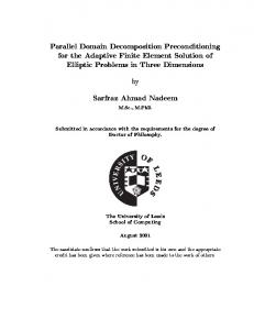
Porous media domain Ω p

Interface Γ

Fluid domain Ω f

Fig. 1.1. The fluid and porous media domains Ωf and Ωp , respectively, an the interface Γ.

Let Γ = Ωp ∩ Ωf denote the interface between the fluid and porous media regions; see Fig. 1.1. Along the interface Γ, we require uf · nf = −up · np , −τ j · (T(uf , pf ) · nf ) = ατ j · uf ,

−nf · (T(uf , pf ) · nf ) = gφp ,

(1.1) (1.2) (1.3)

where nf and np denote the unit outer normal to the fluid and the porous media regions at the interface Γ, respectively; τ j (j = 1, · · · , d−1) denote mutually orthogonal unit tangential vectors to the interface Γ; and the constant parameter α depends on ν and K. The second condition (1.2) is referred to as the Beavers-Joseph-Saffman-Jones (BJSJ) interface condition [12, 19] which is an approximation of the Beavers-Joseph interface boundary condition [1]. The BJSJ boundary condition is also related to the Navier’s slip boundary condition.

A Parallel Robin-Robin Domain Decomposition Method for the Stokes-Darcy System

3

To enable direct comparisons with the results of [8] and for simplicity, we assume that the hydraulic head φp and the fluid velocity uf satisfies homogeneous Dirichlet boundary condition except on Γ , i.e., φp = 0 on the boundary ∂Ωp \Γ and uf = 0 on the boundary ∂Ωf \Γ. The spaces that we utilize are Xf = {vf ∈ [H 1 (Ωf )]d | vf = 0 on ∂Ωf \Γ} Qf = L2 (Ωf ) Xp = {ψp ∈ H 1 (Ωp ) | ψp = 0 on ∂Ωp \Γ}.

For the domain D (D = Ωf or Ωp ), (·, ·)D denotes the L2 inner product on the domain D, and &·, ·' denotes the L2 inner product on the interface Γ or the duality pairing 1/2 between H −1/2 (Γ) and H00 (Γ). With these notations, the weak formulation of the coupled Stokes-Darcy problem is given as follows [2, 8]: find (uf , pf ) ∈ Xf × Qf and φp ∈ Xp such that af (uf , vf ) + bf (vf , pf ) + gap (φp , ψp ) + &gφp , vf · nf ' − &guf · nf , ψp ' +α&Pτ uf , Pτ vf ' = (f , vf )Ωf ∀ vf ∈ Xf , ψp ∈ Xp , bf (uf , qf ) = 0,

∀ qf ∈ Qf ,

(1.4) (1.5)

where the bilinear forms are defined as ap (φp , ψp ) = (K∇φp , ∇ψp )Ωp af (uf , vf ) = 2ν(D(uf ), D(vf ))Ωf bf (vf , q) = −(∇ · vf , q)Ωf and Pτ denoted the projection onto the tangent space on Γ, i.e. Pτ u =

d−1 " j=1

(u · τ j )τ j .

It is easy to see that the system (1.4) and (1.5) is well posed for f ∈ [L2 (Ωf )]d [2, 8]. Since the governing equations are different for the fluid and the porous media region, it is natural to utilize a domain decomposition method so that off-the-shelf efficient solvers for the Darcy system and the Stokes system can be utilized [8]. The central issue is then to determine if the domain decomposition method convergence and its associated convergence rate. The main contribution of this paper is the development and analysis of a new parallel domain decomposition method based on Robin boundary conditions that converges with a rate that, for appropriate choices of acceleration parameters, is independent of the mesh size . For classical second-order elliptic problems, a Robin-type domain decomposition method (DDM) was introduced in [13] where it was also proved that the solution of the Robin DDM converges weakly to the solution of the elliptic problems with respect to the H 1 norm. In [4, 5], new update techniques for the Robin data were introduced and it was proved that the weak convergence in H 1 could induce strong convergence. In [9], it was pointed out that a convergence rate 1 − O(h1/2 ) can be achieved in the case of two subdomains. Recently, a rigorous analysis for the case of many subdomains was given in [16,17] where it was proved, in certain cases such as for a small number of subdomains, that the convergence rate could be 1−O(h1/2 H −1/2 ), where H is the size

4


of the subdomain and h is the size of the finite element grid. In particular, the new term “winding number” was proposed in [17] to describe the depth of subdomains, and in the case of many subdomains and it was shown that the convergence rate not only depends on the mesh size h and the size H of subdomains, but also on the winding number. Furthermore, Robin-type DDMs for parabolic problems was also studied in [18]. In [8], two Robin DDMs for the Stokes-Darcy equations, one a serial version(sRR) and the other a parallel version(pRR), are considered and compared with the DirichletNeumann DDMs [6, 7]; mesh-independent convergence rates were observed for serial Robin DDMs numerically but not proved rigorously. In addition to providing a rigorous analysis, in this paper, we treat the more general case of the Beavers-JosephSaffman-Jones interface boundary condition instead of the further simplified interface boundary conditions considered in [8]. However, the full Beavers-Joseph interface boundary condition is not treated here since well posedness in the steady state case is established only for particular choices of parameters [2]. Other algorithms that combine ideas from multi-grid and DDMs can be found in [14], where the authors proposed to solve the coupled problem directly on a coarse grid (with mesh size hcoarse ) and then use the coarse solution to provide boundary conditions for the Stokes and Darcy systems at the interface so that they may be solved separately on 3 2 ). For DDMs for other settings, a finer mesh (with mesh size of the order of hcoarse and especially for the parallel Robin-Robin domain decomposition methods, one may refer to [4–8, 13, 15–17, 20, 21] and the references cited therein. The rest of the paper is organized as follows. In Section 2, we propose the Robin boundary conditions at the interface for the Stokes and Darcy systems. A necessary and sufficient condition on the equivalence of the Stokes-Darcy system with BeaversJoseph-Saffman-Jones interface boundary condition and the new decoupled Stokes and Darcy systems with Robin boundary conditions is derived. In Section 3, we propose our new parallel Robin-Robin domain decomposition method. We establish the convergence of the new scheme for the case of equal acceleration parameters γf = γp and the case of γf < γp , with a convergence rate for appropriate choices of the acceleration parameters. Finite element approximations are considered in Section 4. In particular, we derive a convergence rate (depending on the mesh size h) for the case of equal acceleration parameters and the case of γp < γf . Although the convergence rate is derived for globally regular triangulations only, we may easily generalize the result to mortar elements so that solvers with different mesh size may be utilized for the fluid and the porous media regions. We present our results of some computational experiments in Section 5. These results are in accordance with our analyses. 2. Robin boundary conditions. In order to solve the coupled Stokes-Darcy problem utilizing the domain decomposition idea, we naturally consider (partial) Robin boundary conditions for the Stokes and the Darcy equations because Robin boundary conditions are more general and embody both the Neumann and Dirichlet type conditions in (1.1)–(1.3). Let us consider the following Robin condition for the Darcy system: for a given constant γp > 0 and a given function ηp defined on Γ, γp K∇φ#p · np + g φ#p = ηp

on Γ.

(2.1)

Then, the corresponding weak formulation for the Darcy system is given by: for


ηp ∈ L2 (Γ), find φ#p ∈ Xp such that

γp ap (φ#p , ψp ) + &g φ#p , ψp ' = &ηp , ψp '

5

∀ ψp ∈ Xp .

Similarly, we propose the following Robin type condition for the Stokes equations: for a given constant γf > 0 and a given function ηf defined on Γ, # f · nf = ηf nf · (T(# uf , p#f ) · nf ) + γf u

on Γ.

(2.2)

Then, the corresponding weak formulation for the Stokes system is given by: for # f ∈ Xf and p#f ∈ Qf such that ηf ∈ L2 (Γ), find u af (# uf , vf ) + bf (vf , p#f ) + γf &# uf · nf , vf · nf ' # f , Pτ vf ' = (f , vf )Ωf + &ηf , vf · nf ' +α&Pτ u bf (# uf , qf ) = 0

∀ qf ∈ Qf .

∀ vf ∈ Xf

(2.3)

We can combine the Stokes and Darcy systems with Robin boundary conditions into one system. Indeed, for any positive constant ω, it is easy to see that if ηp ∈ L2 (Γ) and ηf ∈ L2 (Γ) are given, then, there exists a unique solution (φ#p , u #f , p#f ) ∈ Xp × Xf × Qf such that

af (# uf , vf ) + bf (vf , p#f ) + ωγp ap (φ#p , ψp ) + ω&g φ#p , ψp ' + γf &# uf · nf , vf · nf ' # f , Pτ vf ' = (f, vf )Ωf + &ηf , vf · nf ' + ω&ηp , ψp ' +α&Pτ u ∀ ψp ∈ Xp , vf ∈ Xf bf (# uf , qf ) = 0 ∀ qf ∈ Qf . (2.4) # f , p#f ) is independent of the parameter Remark. 2.1. Note that the solution (φ#p , u ω. Our next goal is to show that, for appropriate choices of γf , γp , ηf , and ηp , (smooth) solutions of the Stokes-Darcy system are equivalent to solutions of (2.4), and hence we may solve the latter system instead of the former. Lemma 2.2. Let (φp , uf , pf ) be the solution of the coupled Stokes-Darcy sys# f , p#f ) be the solution of the decoupled Stokes and Darcy tem (1.4)–(1.5) and let (φ#p , u # f , p#f ) = system with Robin boundary conditions at the interface (2.4). Then, (φ#p , u (φp , uf , pf ) if and only if γf , γp , ηf , and ηp satisfy the following compatibility conditions: # f · nf + g φ#p ηp = γp u # f · nf − g φ#p . ηf = γf u

(2.5) (2.6)

Proof. For the necessity, we set ψp = 0 in the Stokes-Darcy system (1.4)–(1.5) and deduce that (φp , uf , pf ) solves (2.3) if < ηf − γf uf · nf + gφp , vf · nf >= 0

∀ vf ∈ Xf

(2.7)

which implies (2.6). The necessity of (2.5) can be derived in a similar fashion. As for the sufficiency, by setting ω = g/γp in (2.4) and substituting the com# f , p#f ) solves the coupled patibility conditions (2.5)–(2.6), we easily see that (φ#p , u Stokes-Darcy system (1.4)–(1.5). # f , p#f ) = Since the solution to the Stokes-Darcy system is unique, we have (φ#p , u (φp , uf , pf ).

6


3. Robin-Robin domain decomposition methods. 3.1. The Robin-Robin domain decomposition algorithm. Now we propose the following parallel Robin-Robin domain decomposition method for solving the coupled Stokes-Darcy system. 1. Initial values of ηp0 and ηf0 are guessed. They may be taken to be zero. 2. For k = 1, 2, . . ., independently solve the Stokes and Darcy systems with Robin boundary conditions. More precisely, φkp ∈ Xp is computed from γp ap (φkp , ψp ) + &gφkp , ψp ' = &ηpk , ψp '

∀ ψp ∈ Xp ;

(3.1)

and ukf ∈ Xf and pkf ∈ Qf are computed from af (ukf , vf ) + bf (vf , pkf ) + γf &ukf · nf , vf · nf ' + α&Pτ ukf , Pτ vf ' bf (ukf , qf )

=0

= &ηfk , vf · nf ' + (f , vf )Ωf

∀ vf ∈ Xf ,

∀ qf ∈ Qf .

(3.2) (3.3)

3. ηpk+1 and ηfk+1 are updated in the following manner: ηfk+1 = aηpk + bgφkp

(3.4)

ηpk+1 = cηfk + dukf · nf

(3.5)

where the coefficients a, b, c, d are chosen as follows: γf b = −1 − a γp c = −1 d = γf + γp .

a=

(3.6) (3.7)

In the special case for which γf = γp = γ, we have b = −2

a=1

c = −1

d = 2γ.

The relations (3.6)–(3.7) are necessary to ensure the convergence of the scheme. Indeed, suppose that ηfk and ηpk converge to ηf∗ and ηp∗ , respectively, and φkp , ukf also converge to the true solution φ∗p and u∗f , respectively. Then, by (3.4)–(3.5) and Lemma 2.2, we see that the following relationships hold: ηf∗ = aηp∗ + bgφ∗p = γf u∗f · nf − gφ∗p , ηp∗

This leads to $

bgφ∗p du∗f · nf

%

= =

=

cηf∗

+

du∗f

$

b 0

0 d

%$

$

1 −c

· nf =

γp u∗f

· nf +

gφ∗p .

% $ %$ ∗ % gφ∗p ηf 1 −a = u∗f · nf −c 1 ηp∗ % %$ %$ gφ∗p −a −1 γf ∗ uf · nf 1 1 γp

(3.8) (3.9)

(3.10)

which implies the consistency equations (3.6)–(3.7) on the coefficients a, b, c, d and γf , γp . These relationships (3.6)–(3.7) among the parameters are used in the convergence analysis of the Robin-Robin domain decomposition method.


7

Remark. 3.1. If the updating strategy (3.4)–(3.5) is changed to ηfk+1 = a1 ηpk + b1 gφkp + c1 ukf · nf

ηpk+1 = a2 ηfk + b2 gφkp + c2 ukf · nf , then, the “consistency” conditions change to $ %$ % $ −a1 1 1 γp b1 = 1 a2 −1 γf b2

c1 c2

%

.

In this case, we have more flexibility. However, the convergence analysis is somewhat more complicated, and will be addressed elsewhere. The parallel Robin-Robin domain decomposition algorithm proposed here is related to the serial version (sRR algorithm) of [8]. As a matter of fact, the sRR algorithm can be obtained by implementing our algorithm serially as follows. Initialize ηp0 , and, for k = 0, 1, . . . , 1. Find φkp by solving the Darcy system (3.1). 2. Set ηfk = aηpk + bgφkp and find ukf and pkf by solving the Stokes system (3.2)– (3.3). 3. Set ηpk+1 = cηfk + dukf · nf . In [8], it is proved, for γf = γp = γ, that the solution of the sRR algorithm converges to the solution of the Darcy-Stokes systems. Here, we are able to prove a similar convergence result. Moreover, we are able to demonstrate that the convergence could be geometric for appropriate choice of γf < γp . 3.2. Convergence of the parallel Robin-Robin DDM. We follow the elegant energy method proposed in [13] to demonstrate the convergence of the parallel Robin-Robin domain decomposition method for appropriate choice of parameters γp and γf . To this end, let (φp , uf , pf ) denote the solution of the coupled Stokes-Darcy system (1.4)–(1.5). Then, we have that (φp , uf , pf ) solves the equivalent decoupled system (2.4) with γf , γp , ηp , ηf satisfying the compatibility conditions (2.5)–(2.6) with the hats removed. Next, we define the error functions )kp = ηp − ηpk

ekφ = φp − φkp

)kf = ηf − ηfk

eku = uf − ukf

ekp = pf − pkf .

Then, the error functions satisfy the following error equations: γp ap (ekφ , ψp ) + &gekφ , ψp ' = &)kp , ψp '

∀ ψp ∈ Xp ,

af (eku , vf ) + bf (vf , ekp ) + γf &eku · nf , vf · nf ' + α&Pτ eku , Pτ vf ' bf (eku , qf )

=0

= &)kf , vf · nf ' ∀ qf ∈ Qf ,

∀ vf ∈ Xf ,

(3.11)

(3.12) (3.13)

and, along the interface Γ, )k+1 = a)kp + bgekφ f

(3.14)

)k+1 = c)kf + deku · nf . p

(3.15)

8


Equation (3.15) leads to *)k+1 *2Γ = c2 *)kf *2Γ + d2 *eku · nf *2Γ + 2cd&)kf , eku · nf '. p Setting vf = eku in (3.12), we deduce &)kf , eku · nf ' = af (eku , eku ) + γf *eku · nf *2Γ + α*Pτ eku *2Γ and, hence, combining the last two equations, we have *)k+1 *2Γ = c2 *)kf *2Γ + (d2 + 2cdγf )*eku · nf *2Γ + 2cd af (eku , eku ) + 2cd α*Pτ eku *2Γ . (3.16) p Similarly, (3.14) implies *)k+1 *2Γ = a2 *)kp *2Γ + b2 *gekφ *2Γ + 2ab&)kp , gekφ '. f Setting ψp = gekφ in (3.11), we have &)kp , gekφ ' = γp ap (ekφ , gekφ ) + &gekφ , gekφ '. Combining the last two equations, we deduce *)k+1 *2Γ = a2 *)kp *2Γ + (b2 + 2ab)*gekφ*2Γ + 2abγp g ap (ekφ , ekφ ). f

(3.17)

Substituting (3.6)–(3.7) into (3.16) and (3.17), we have the following result. Lemma 3.2. The error functions satisfy *)k+1 *2Γ = *)kf *2Γ + (γp2 − γf2 )*eku · nf *2Γ p

−2(γf + γp )af (eku , eku ) − 2(γf + γp ) α*Pτ eku *2Γ & $ %2 % $ %2 ' $ γf γf γf k+1 2 k 2 *)f *Γ = *)p *Γ + 1 − *gekφ *2Γ − 2γf 1 + g ap (ekφ , ekφ ). γp γp γp We are now ready to demonstrate the convergence of our parallel Robin-Robin domain decomposition method. The convergence analysis for γf = γp and γf += γp are different and will be treated separately. Case 1: γf = γp = γ. In this case, we have *)k+1 *2Γ = *)kf *2Γ − 4γaf (eku , eku ) − 4γα*Pτ eku *2Γ p

*)k+1 *2Γ = *)kp *2Γ − 4γgap (ekφ , ekφ ). f

Adding the two equations and summing over k from k = 0 to N , we deduce +1 2 +1 2 *)N *Γ + *)N *Γ = *)0p *2Γ + *)0f *2Γ − 4γ p f

N "

k=0

(af (eku , eku ) + g ap (ekφ , ekφ ) + α*Pτ eku *2Γ ).

+1 2 +1 2 This implies that *)N *Γ + *)N *Γ is bounded from above by *)0p *2Γ + *)0f *2Γ and p f that eku and ekφ tend to zero in (H 1 (Ωf ))d and H 1 (Ωp ), respectively. The convergence 1 of ekφ together with the error equation (3.11) implies the convergence of )kp in H − 2 (Γ). Combining the convergence of )kp and ekφ and the error equation on the interface (3.14), 1 we deduce the convergence of )kf in H − 2 (Γ). The convergence of the pressure then


9

follows from the inf-sup condition and (3.12)–(3.13). Note that we have no rate of convergence here. Hence, we have proved the following result. Theorem 3.3. If γp = γf = γ, then Xp

φkp −→ φp

Xf

ukf −→ uf

Qf

pkf −→ pf ,

and 1

H − 2 (Γ)

ηpk

−→ γuf · nf + gφp = −γK∇φp · np + gφp

1

ηfk

H − 2 (Γ)

−→ γuf · nf − gφp = nf · (T(uf , pf ) · nf ) + γuf · nf .

Case 2: γf < γp . In this case, because ekφ ∈ Xp , we deduce that, thanks to the trace theorem and the Poincaré inequality, there exists a constant Cp (independent of K) such that *ekφ *2Γ ≤ Cp *K−1 *ap (ekφ , ekφ ).

(3.18)

1 1 2 − ≤ , γf γp gCp *K−1 *

(3.19)

Thus, if γf < γp and

we have &

$

%2 '

$ % γf 1− − 2γf 1 + gap (ekφ , ekφ ) γp $ % $$ % % γf 1 1 −1 ≤ γf g 1 + − gCp *K * − 2 ap (ekφ , ekφ ) γp γf γp ≤ 0. γf γp

*gekφ *2Γ

Similarly, thanks to the trace theorem and Korn’s inequality, there exists a constant Cf such that ( *eku · nf *2Γ ≤ Cf |D(eku )|2 dx. Ωf

Therefore, under the additional constraint γp − γf ≤

4ν , Cf

we have (γp2 − γf2 )*eku · nf *2Γ ≤ 2(γf + γp )af (eku , eku ). Hence we have, when combined with Lemma 3.2, *)k+1 *2Γ ≤ *)kf *2Γ , p

*)k+1 *2Γ ≤ f

$

γf γp

%2

*)kp *2Γ

(3.20)

10


which leads to *)k+1 *Γ ≤ p

γf k−1 *) *Γ , γp p

*)k+1 *Γ ≤ f

γf k−1 *) *Γ . γp f

This implies the convergence of the η which further implies the convergence of the velocity eku , the pressure ekp , and the hydraulic head ekφ through the error equations (3.11) and (3.12)–(3.13). Hence we have derived the following geometric convergence result. Theorem 3.4. Assume that the parameters γp and γf are chosen so that 0 < γp − γf ≤

4ν Cf

1 1 2 − ≤ . γf γp gCp *K−1 *

(3.21)

Then, the solutions of the parallel Robin-Robin domain decomposition method converge to the solution of the Stokes-Darcy system. Moreover, ap (ekφ , ekφ )

+

af (eku , eku )

+

*ekp *2Γ

+

*)kp *2Γ

+

*)kf *2Γ

≤C

$

γf γp

%# k2 $

* ) 0 2 *)p *Γ + *)0f *2Γ .

The last inequality follows from the geometric convergence of )kp , )kf , the error relationship at the interface and the error equations. 4. Finite element approximations. We next consider finite element discretization of the Robin domain decomposition method that was proposed in the previous section. One of the advantages of considering finite element approximations is that we can then derive explicit convergence rates, even for the case γf = γp = γ. Of course, the rate of convergence will depend on the size of the element h. This is different from the case of γf < γp where the rate of convergence is independent of h. We will also demonstrate the convergence of the finite element approximation even in the parameter region of γp < γf which may seem unlikely in view of Lemma 3.2. One of the key advantages of the finite element setting is the availability of an inverse Poincaré type inequality [3] that allows us to control various terms. ! We consider a regular triangulation Th of the global domain Ωp Ωf which is assumed to be regular and quasi-uniform. We also assume that the triangulation Tf,h , Tp,h induced on the subdomains Ωf and Ωp are compatible on Γ and the mesh on the interface Γ is quasi-uniform. The induced triangulation on Γ will be denoted Bh . Non-matching grid or mortar cases will be considered elsewhere. We denote by Xp,h ⊂ Xp a finite element space on the porous media domain Ωp and denote by Xf,h ⊂ Xf and Qf,h ⊂ Qf finite element spaces on the fluid domain Ωf . We use these spaces to approximate the hydraulic head in the porous media and the fluid velocity and pressure. Specifically, we choose + + + 0 Xp,h = {ψp,h ∈ C (Ωp ) ++ ψp,h |T ∈ P2 (T ), ∀ T ∈ Tp,h , ψp,h +∂Ωp \Γ = 0} + + + Xf,h = {vf,h ∈ (C 0 (Ωf ))d ++ vf,h |T ∈ (P2 (T ))d , ∀ T ∈ Tf,h , vf,h +∂Ω \Γ = 0} f + + Qf,h = {qp,h ∈ C 0 (Ωf ) ++ qf,h |T ∈ P1 (T ), ∀ T ∈ Tf,h }.


11

The spaces Xf,h and Qf,h are assumed to satisfy the discrete LBB or inf-sup condition [10, 11]. We also define the discrete trace space on the interface + + 0 Zh = {ηh ∈ C (Γ) ++ ηh |τ ∈ P2 (τ ), ∀ τ ∈ Bh , ηh |∂Γ = 0}. It is easy to see that Zh is the trace space in the sense that + Yp,h : = Xp,h +Γ = Zh , + Yf,h : = Xf,h + · nf = Zh . Γ

The discrete weak formulation of the coupled Stokes-Darcy problem is then given by: find (uf,h , pf,h ) ∈ Xf,h × Qf,h and φp,h ∈ Xp,h such that af (uf,h , vf ) + bf (vf , pf,h ) + gap (φp,h , ψp ) + &gφp,h , vf · nf ' − &guf,h · nf , ψp ' +α&Pτ uf,h , Pτ vf ' = (f , vf )Ωf ∀ vf ∈ Xf,h , ψp ∈ Xp,h bf (uf,h , qf ) = 0, ∀ qf ∈ Qf,h . (4.1) The FEM approximation of the decoupled Stokes-Darcy system with Robin boundary conditions (2.1)–(2.2) can be formulated in the following way: for given ηp,h ∈ # f,h , p#f,h ) ∈ Xp,h × Xf,h × Qf,h such that L2 (Γ) and ηf,h ∈ L2 (Γ), find (φ#p,h , u

af (# uf,h , vf ) + bf (vf , p#f,h ) + ωγp ap (φ#p,h , ψp ) + ω&g φ#p,h , ψp ' + γf &# uf,h · nf , vf · nf ' # f,h , Pτ vf ' = (f , vf )Ωf + &ηf,h , vf · nf ' + ω&ηp,h , ψp ', +α&Pτ u ∀ ψp ∈ Xp,h , vf ∈ Xf,h bf (# uf,h , qf ) = 0, ∀ qf ∈ Qf,h . (4.2) Similar to the continuous case, finite element approximations of the coupled Stokes-Darcy system, defined by (4.1), and of the revised Robin approximation, defined by (4.2), are related in the following fashion: # f,h , p#f,h ) = (φp,h , uf,h , pf,h ) Lemma 4.1. For ηp,h ∈ Yp,h and ηf ∈ Yf,h , (φ#p,h , u if and only if ηp,h and ηf,h satisfy ηp,h = Pp,h (γp uf,h · nf + gφp,h )

ηf,h = Pf,h (γf uf,h · nf − gφp,h ),

where Pp,h and Pf,h are L2 (Γ)-projections onto the spaces Yp,h and Yf,h respectively, i.e., for v ∈ L2 (Γ), &Pp,h v, wp ' = &v, wp '

∀ wp ∈ Yp,h

&Pf,h v, wf ' = &v, wf '

∀ wf ∈ Yf,h .

Remark. 4.2. Comparing with the Robin conditions (2.1) and (2.2), we see that we have heuristically used Pp,h (γp K∇φp,h · np + gφp,h ) = ηp,h Pf,h (nf · (T (uf,h , pf,h ) · nf ) + γf uf,h · nf ) = ηf,h . The choices of the spaces Yp,h and Yf,h are not unique; other choices are also possible. The parallel Robin-Robin domain decomposition finite element method is defined as follows. 0 0 1. The initial values of ηp,h ∈ Yp,h and ηf,h ∈ Yf,h are guessed; they may be taken to be zero.

12


2. For k = 1, 2, . . ., solve the discrete Stokes and Darcy systems with Robin conditions independently, i.e., φkp,h ∈ Xp,h is determined from k , ψp ' γp ap (φkp,h , ψp ) + &gφkp,h , ψp ' = &ηp,h

∀ ψp ∈ Xp,h ;

and ukf,h ∈ Xf,h and pkf,h ∈ Qf,h are determined from af (ukf,h , vf ) + bf (vf , pkf,h ) + γf &ukf,h · nf , vf · nf ' + α&Pτ ukf,h , Pτ vf ' k , vf · nf ' + (f , vf )Ωf = &ηf,h

bf (ukf,h , qf )

∀ vf ∈ Xf,h

∀ qf ∈ Qf,h .

=0

k+1 k+1 3. ηp,h and ηf,h are updated by k+1 k + bgφkp,h ) ηf,h = Pf,h (aηp,h

k+1 k + dukf · nf ). ηp,h = Pp,h (cηf,h

+ + k k One important observation is that ηp,h , ηf,h , φkp,h +Γ , ukf · nf +Γ ∈ Zh for all k, provided that the initial guesses belong to Zh . Therefore, the projections Pp,h and Pf,h in the implementation of the algorithm are identity operators. We now consider the error functions for finite element approximations, just as in the continuous case studied in the previous section. Let k )kp,h = ηp,h − ηp,h

ekφ,h = φp,h − φkp,h

k )kf,h = ηf,h − ηf,h ,

eku,h = uf,h − ukf,h

ekp,h = pf,h − pkf,h .

It is straightforward to verify that )kp,h ∈ Zh

)kf,h ∈ Zh

ekφ,h |Γ ∈ Zh

eku,h · nf ∈ Zh .

It is also easy to see that the error functions satisfy the error equations γp ap (ekφ,h , ψp ) + &gekφ,h , ψp ' = &)kp,h , ψp '

∀ ψp ∈ Xp,h ,

af (eku,h , vf ) + bf (vf , ekp,h ) + γf &eku,h · nf , vf · nf ' + α&Pτ ekf,h , Pτ vf ' = &)kf,h , vf · nf '

bf (eku,h , qf )

=0

∀ vf ∈ Xf,h

∀ qf ∈ Qf,h ,

(4.3)

(4.4) (4.5)

and, along the interface, k k )k+1 f,h = Pf,h (a)p,h + bgeφ,h )

k k )k+1 p,h = Pp,h (c)f,h + deu,h · nf ).

It is easy to verify the following relationship for the error functions, just as in the continuous case. Lemma 4.3. The error functions satisfy 2 k 2 2 2 k 2 k k k 2 *)k+1 p,h *Γ = *)f,h *Γ + (γp − γf )*eu,h · n*Γ − 2(γf + γp )af (eu,h , eu,h ) − 2(γf + γp )*Pτ eu,h *Γ & $ %2 $ %2 ' $ % γf γf γf k+1 2 k 2 k 2 *)f,h *Γ = *)p,h *Γ + 1 − *geφ,h*Γ − 2γf 1 + gap (ekφ,h , ekφ,h ). γp γp γp

13


The key ingredient in deriving an explicit convergence rate for the case of γf = γp is the following estimate. Lemma 4.4. *)kp,h *2Γ ≤ C(*K−1 *1/2 + γp h−1/2 *K*1/2 )2 ap (ekφ,h , ekφ,h ). Proof. The key in the proof of this lemma is an extension operator. Let Np,h be the set of nodes for the finite element triangulation on Ωp , and let Np,Γ = Np,h |Γ . Denote Ep,h the zero extension operator from Yp,h = Zh to Xp,h : , k )p,h (P ) if P ∈ Np,Γ Ep,h )kp,h (P ) = 0 if P ∈ Np,h \Np,Γ . Then, we have *Ep,h )kp,h *2L2 (Ωp ) ≈ hd

"

P ∈Np,h

(Ep,h )kp,h (P ))2 ≈ hd

"

P ∈Np,Γ

()kp,h (P ))2 ≈ h*)kp,h *2Γ . (4.6)

Note that Ep,h )kp,h ∈ Xp,h due to the definition of the extension operator and the fact that )kp,h ∈ Zh . Hence, we may set ψp = Ep,h )kp,h in (4.3) and utilize Cauchy-Schwarz inequality to deduce *)kp,h *2Γ = γp ap (ekφ,h , Ep,h )kp,h ) + &gekφ,h , )kp,h '

≤ γp ap (ekφ,h , ekφ,h )1/2 ap (Ep,h )kp,h , Ep,h )kp,h )1/2 + *gekφ,h*Γ *)kp,h *Γ . (4.7)

On the other hand, thanks to the inverse inequality for finite element spaces and (4.6), we deduce ap (Ep,h )kp,h , Ep,h )kp,h ) ≤ *K**∇Ep,h )kp,h *2L2 (Ωp )

≤ Ch−2 *K**Ep,h)kp,h *2L2 (Ωp ) ≤ Ch−1 *K**)kp,h*2Γ .

(4.8)

Combining the inequality (3.18) with (4.7)–(4.8), we obtain *)kp,h *2Γ ≤ Cγp h−1/2 *K*1/2 ap (ekφ,h , ekφ,h )1/2 *)kp,h *Γ +Cp1/2 *K−1 *1/2 ap (ekφ,h , ekφ,h )1/2 *)kp,h *Γ which implies the lemma. Remark. 4.5. Similar results are available for P1 conforming and nonconforming elements for classical second-order elliptic problems( [16, 17]). Now for γf = γp = γ, by Lemma 4.3, we have 2 k 2 k k k 2 *)k+1 p,h *Γ = *)f,h *Γ − 4γaf (eu,h , eu,h ) − 4γ*Pτ eu,h *Γ 2 k 2 k k *)k+1 f,h *Γ = *)p,h *Γ − 4γgap (eφ,h , eφ,h ).

Combining the above equalities with Lemma 4.4, we deduce 2 k 2 *)k+1 p,h *Γ ≤ *)f,h *Γ ,

1

2 −1 1/2 *)k+1 * + γh− 2 *K*1/2 )−2 )*)kp,h *2Γ . f,h *Γ ≤ (1 − Cγ(*K

Therefore, we have proved the following lemma. Lemma 4.6. For γf = γp = γ, we have 2 −1 1/2 2 *)k+1 * + γh−1/2 *K*1/2 )−2 )*)k−1 p,h *Γ ≤ (1 − Cγ(*K p,h *Γ

2 −1 1/2 2 *)k+1 * + γh−1/2 *K*1/2 )−2 )*)k−1 f,h *Γ ≤ (1 − Cγ(*K f,h *Γ .

14


This further implies convergence with convergence rate proportional to 1 − Ch1/2 for the case of γp = γf = γ. Theorem 4.7. If γp = γf = γ, then ap (ekφ,h , ekφ,h ) + af (eku,h , eku,h ) + *ekp,h *2L2 (Ωf ) + *)kp,h *2Γ + *)kf,h *2Γ

* k ) ≤ C(1 − Cγ(*K−1 *1/2 + γh−1/2 *K*1/2 )−2 )# 2 $ *)0p *2Γ + *)0f *2Γ .

Remark. 4.8. One important question is how to choose the parameter γ so that the Robin-Robin domain decomposition method has fast/optimal convergence rate. The analysis above suggests that the optimal choice of the parameter may depend on both the mesh grid size h and the hydraulic conductivity tensor K. One possible choice of γ is to balance the terms γ −1 *K−1 * and γh−1 *K* and let γ=

&K−1 &1/2 h1/2 . &K&1/2

Then,

γ h1/2 = . (*K−1 *1/2 + γh−1/2 *K*1/2 )2 *K−1 *1/2 *K*1/2

(4.9)

Now, if we assume that K = KI, then *K−1 *1/2 *K*1/2 = 1, so the convergence rate of the Robin-Robin domain decomposition finite element method is 1 − Ch1/2 . In the case γf += γp , we have the same result as Theorem 3.4 with geometric convergence with rate independent of h. Theorem 4.9. If (3.21) is satisfied, then ap (ekφ,h , ekφ,h )+af (eku,h , eku,h )+*ekp,h *2L2 (Ωf ) +*)kp,h *2Γ +*)kf,h *2Γ ≤ C

$

γf γp

%k

) 0 2 * *)p,h *Γ + *)0f,h *2Γ .

Now we consider the case γf > γp which is counter-intuitive in view of Lemma 3.2. Nevertheless, at the discrete level, we are able to control the excessive growth term by the decay terms so long as the parameters γf and γp are chosen to be close (depending on K and h). Indeed, thanks to Lemma 4.4, we have % $ γf γf ( )2 − 1 *)kp,h *2Γ − γf (1 + )g ap (ekφ,h , ekφ,h ) γp γp % $ γf γf 2 ≤ (( ) − 1)C(*K−1 *1/2 + γp h−1/2 *K*1/2 )2 − γf (1 + )g ap (ekφ,h , ekφ,h ) γp γp $ % 1 1 γf = γf (1 + ) ( − )C(*K−1 *1/2 + γp h−1/2 *K*1/2 )2 − g ap (ekφ,h , ekφ,h ) γp γp γf ≤0 provided that the following condition holds 0≤

1 g 1 − ≤ . γp γf C(*K−1 *1/2 + γp h−1/2 *K*1/2 )2

(4.10)

An undesirable feature here is the dependence on the mesh size h. For every small h, the γs must be very close in order to have the above inequality satisfied. This would lead to a very slow convergence rate.


15

We then have, when combined with Lemma 4.3 and under the assumption (4.10), k 2 k k k k k 2 2 *)k+1 p,h *Γ ≤ *)f,h *Γ − 2(γf + γp )af (eu,h , eu,h ) ≤ *)f,h *Γ − 4γp af (eu,h , eu,h ) $ % γf 2 2 k *)k+1 g ap (ekφ,h , ekφ,h ) ≤ *)kp,h *2Γ − 2γf g ap (ekφ,h , ekφ,h ). f,h *Γ ≤ *)p,h *Γ − γf 1 + γp

Summing the two inequalities for k from 0 to N , we deduce the convergence of ekφ,h and eku,h that leads to the convergence (without rate) of all quantities involved. A rate of convergence can be derived just as in the case of γp = γf . Indeed, we may deduce, with the help of Lemma 4.4 and the last inequality above, 2 −1 1/2 * + γp h−1/2 *K*1/2 )−2 )*)kp,h *2Γ *)k+1 f,h *Γ ≤ (1 − Cγf (*K

and hence we obtain 2 −1 1/2 2 * + γp h−1/2 *K*1/2 )−2 )*)k−1 *)k+1 p,h *Γ p,h *Γ ≤ (1 − Cγf (*K

2 −1 1/2 2 *)k+1 * + γp h−1/2 *K*1/2 )−2 )*)k−1 f,h *Γ ≤ (1 − Cγf (*K f,h *Γ .

This further implies convergence with convergence rate proportional to 1 − Ch1/2 for the case of γp < γf under the additional constraint of (4.10). Therefore, we have proved the following theorem. Theorem 4.10. For γp < γf , assume that the additional constraint (4.10) holds. Then, we have the following convergence result for our parallel Robin-Robin domain decomposition finite element methods for the coupled Stokes-Darcy system: ap (ekφ,h , ekφ,h ) + af (eku,h , eku,h ) + *ekp,h *2L2 (Ωf ) + *)kp,h *2Γ + *)kf,h *2Γ

* k ) ≤ C(1 − Cγf (*K−1 *1/2 + γp h−1/2 *K*1/2 )−2 )# 2 $ *)0p *2Γ + *)0f *2Γ .

5. Computational experiments. We present some preliminary computational results based on the parallel Robin-Robin domain decomposition finite element method for the coupled Stokes-Darcy system with Beavers-Joseph-Saffman-Jones interface boundary condition. In order to make direct comparisons with [8], we also present computational results for the simplified boundary condition τ j · uf = 0 used in that paper instead of the Beavers-Joseph-Saffman-Jones interface boundary condition (1.2). This simplified interface boundary condition can be formally derived in the limit of α → ∞ in (1.2). We consider two test problems. The first is the example from [8]. Example 1: Let Ωp = (0, 1) × (0, 1), Ωf = (0, 1) × (1, 2), and Γ = {0 ≤ x ≤ 1, y = 1}. The exact solution is given by (uf )1 = y 2 − 2y + 1

(uf )2 = x2 − x

p = 2ν(x + y − 1) + 1/(3K) φ = (x(x − 1)(y − 1) +

y3 − y 2 + y)/K + 2xν. 3

The data in the Stokes-Darcy problem is manufactured using this exact solution. The second test problem is physically more realistic.

16


Example 2: Let Ωp = (0, π) × (−1, 0), Ωf = (0, π) × (0, 1), and Γ = {0 ≤ x ≤ π, y = 0}. Let v(y) denote any function that satisfies the boundary conditions v(0) = −2K and v ' (0) = 0 and let uf,1 = v ' (y) cos x

uf,2 = v(y) sin x

pf = 0

φp = (ey − e−y ) sin x.

Assume that the hydraulic conductivity is homogeneous and isotropic, i.e., K = KI. Then, for any v(y) satisfying the boundary conditions v(0) = −2K and v ' (0) = 0, these functions exactly satisfy the Stokes-Darcy system with the simplified interface condition (5) (but with inhomogeneous Dirichlet boundary condition on ∂Ω). For example, we may take v(y) = −2K + c sin2 (πy). If c = πK2 , then these functions also satisfy the Beavers-Joseph-Saffman-Jones interface boundary condition with any α. The data in the Stokes-Darcy problem is manufactured using these function as the exact solution. Remark. 5.1. More complex versions of Example 2 can be easily constructed. For instance, a nontrivial pressure field can be considered by simply making sure that pf (x, 0) = 0 and then update the body force f accordingly. We may even construct an exact solution for which the homogeneous boundary condition for the hydraulic head φp is satisfied at the expense of introducing an additional (artificial) body force for the Darcy system. Additional examples satisfying the Beavers-JosephSaffman-Jones interface boundary condition (1.2) instead of the simplified interface boundary condition (5) can be derived easily as well. One merely needs to arrange for v(0) = −2K, v ' (0) = 0, and v '' (0) = 2K as in example 2. Alternatively, we could set v(y) = −2K + Ky 2 + cy 3 in example 2. For domains with flat boundaries, we may also use symbolic computational tools to find exact solutions (even with Beavers-JosephSaffman-Jones interface boundary condition) that are quadratic in the velocity, linear in the pressure, and cubic in the hydraulic head. Example 1 is a special case. 5.1. Convergence of the finite element method. Here we address the issue of the convergence of the finite element method, i.e., we directly solve the full coupled Stokes-Darcy system without using domain decomposition. Recall that we use P2 elements to approximate φp on the domain Ωp and the Hood-Taylor element pair ((P2 )2 for uf and P1 for pf ) on the domain Ωf . We use a uniform triangular meshes constructed by subdividing the rectangular domain Ω into squares of side h and then dividing each square into two triangles. We compute the finite element approximation using the sequence of grid sizes h = 2m , m = 1, . . . , 6. Errors are measured using the discrete ,2 norm which is proportional to the L2 (Ωf ) error, modulo a factor of h2 . We presume that the relative error in the approximation to the velocity in the fluid satisfies $ %α 1 *uf − uf,m * α ≈ Ch = C relative error = *uf * 2m for some α, where uf,m denotes the finite element approximation obtained with h = 2−m . Then, we have that log(relative error) = log

*uf − uf,m * ≈ log C − mα log 2 *uf *

and convergence factor =

*uf − uf,m * = 2α . *uf − uf,m+1 *

17


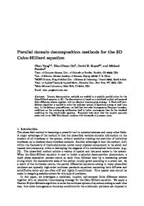
In Figures 5.1 and 5.3, the log of the relative error and the convergence factor are plotted versus m. Similar plots are given for φp in Figures 5.2 and 5.4. Since we are using quadratic finite element spaces for both φp and uf , we expect that α = 3 so that we expect a convergence factor of 8 and a slope in the relative error curve equal to 3 log 2. There are a two noteworthy observations that may be gleaned from the computational results. • The convergence rates depend on the parameters K and ν. • For the case K = KI and ν = 1, it seems that we have super-convergence, i.e., *φp − φp,h * ≈ O(h3.5 ). *φp,h *

*uf − uf,h * ≈ O(h3.5 ) *uf,h * error of finite element solution, norm(u−uh)/norm(u)

0

convergence rate of u

10

16 K=1 K=10−2

−1

10

K=10−4

14

−6

K=10 −2

10

12 −3

10

10 −4

10

8

−5

K=1

10

−2

K=10 10

K=10−6

−7

10

K=10−4

6

−6

1

2

3 4 Example 2, ν=1, n=[2 4 8 16 32 64]

5

6

4

1

1.5

2

2.5 3 3.5 4 Example 2, ν=1, n=[2 4 8 16 32 64]

4.5

5

Fig. 5.1. Relative error (left) and convergence factor (right) of the finite element approximation of uf versus m for Example 2 with ν = 1.

5.2. Convergence of the Robin-Robin domain decomposition method. We now consider the differences between iterations of the Robin-Robin domain decomposition method and the exact solution of the discrete finite element problems. Specifically, in the figures that follow, we plot the ,2 norm of (ukf,h − uf,h ) versus the iteration counter k. The computational results presented confirm our theoretical convergence analysis. By setting K = 1, ν = 1 and γf = 1, Figure 5.5 shows that, for the parallel Robin-Robin domain decomposition method, • if γf < γp (γp = 13 γf or 12 γf ), convergence is very fast; the error is reduced by a factor of γf /γp every two steps; • if γf > γp (γp = 3γf or 2γf ), the iterative method diverges; • if γf = γp , the iterative method converges, but with a slow rate. It is interesting to compare the parallel and serial versions of the Robin-Robin domain decomposition method. Note that the serial version of our algorithm is just the sRR algorithm of [8]. Figure 5.6 shows the results for the serial version. Comparing with Figure 5.5, we see that the behaviors of the two methods are similar except that

18

W. Chen, G. Max, X. Wang error of finite element solution, norm(φ−φh)/norm(φ)

1

convergence rate of φ

10

18 K=1

K=1 −2

K=10

0

10

K=10−2

16

−4

K=10−4

K=10

K=10−6

−1

10

−2

10

12

−3

10

10

−4

10

8

−5

10

6

−6

10

4

−7

10

−6

K=10

14

1

2

3 4 Example 2, ν=1, n=[2 4 8 16 32 64]

5

6

2

1

1.5

2

2.5 3 3.5 4 Example 2, ν=1, n=[2 4 8 16 32 64]

4.5

5

Fig. 5.2. Relative error (left) and convergence factor (right) of the finite element approximation of φp versus m for Example 2 with ν = 1. error of finite element solution, norm(u−uh)/norm(u)

−1

convergence rate of u

10

16 K=1

K=1

K=10−2 −2

−4

10

K=10−2

14

K=10

K=10−4

−6

K=10

K=10−6

−3

10

12

−4

10

10

−5

10

8

−6

10

6

−7

10

1

2

3

4 −6

Example 2, ν=10 , n=[2 4 8 16 32 64]

5

6

4

1

1.5

2

2.5

3

3.5

4

4.5

5

Example 2, ν=10−6, n=[2 4 8 16 32 64]

Fig. 5.3. Relative error (left) and convergence factor (right) of the finite element approximation of uf versus m for Example 2 with ν = 10−6 .

the error for the serial version reduces or increases about two times faster, as the case may be, than the error for the parallel version. √ 5.3. Possible choice of γ. In (4.9), we point that γ can be chosen as γ = h/K which leads to same convergence rate for different K = KI. We set the parameters ν = 1, K = 1, 10−2 , 10−4 , 10−6 , 102 , 104 , 106 . Figure 5.7 shows that the convergence rates are similar; for large K, the convergence rates are same. Note that the exact solution depends on the parameters ν and K, therefore the errors of the initial step are different, so it is better to compare the decreased speed of the error. 5.4. The choice of the parameters γf and γp . It is interesting to point out that our scheme converges in the case of γf ≤ γp which is contrary to [8]. In fact,

19

A Parallel Robin-Robin Domain Decomposition Method for the Stokes-Darcy System error of finite element solution, norm(φ−φ )/norm(φ)

convergence rate of φ

h

−1

10

18 K=1 −2

K=10

−2

10

−4

17

K=10

K=10−6 −3

10

16 −4

10

15 −5

10

14

−6

K=1

10

K=10−2

10

−6

K=10

−8

10

K=10−4

13

−7

1

2

3

4

5

12

6

1

1.5

Example 2, ν=10−6, n=[2 4 8 16 32 64]

2

2.5

3

3.5

4

4.5

5

Example 2, ν=10−6, n=[2 4 8 16 32 64]

Fig. 5.4. Relative error (left) and convergence factor (right) of the finite element approximation of φp versus m for Example 2 with ν = 10−6 .

error of Robin DDM solution with finite element solution, |uk− uh|2

4

10

2

10

0

10

−2

10

−4

10

γ =1/3γ

−6

p

10

f

γp=1/2γf −8

γp=γf

10

γ =2γ p

−10

10

f

γp=3γf

−12

10

0

5

10 15 20 K=1, ν=1, γ =1/K, h=1/32

25

30

f

Fig. 5.5. Error in the iterates versus the iteration counter k for the parallel Robin-Robin domain decomposition method.

for their choice of acceleration parameters γf = 0.3, γp = 0.1, we observe numerical instability of the iterative process. The parameters γf and γp should be chosen carefully. Let us repeat the numerical experiments in [8], where the sRR algorithm(i.e. the serial version of our Robin-Robin algorithm) shows very attractive results for γf = 0.3, γp = 0.1. However, the results

20



15

10

γp=1/3γf γ =1/2γ

10

p

10

f

γp=γf γp=2γf

5

10

γ =3γ p

f

0

10

−5

10

−10

10

−15

10

0

5

10 15 20 K=1, ν=1, γ =1/K, h=1/32

25

30

f

Fig. 5.6. Error in the iterates versus the iteration counter k for the serial Robin-Robin domain decomposition method.

0

−2

10

10 K=1 K=10−2 K=10−4

−1

10

−4

10

K=10−6 2

K=10

4

K=10

−2

−6

K=106

10

10

−3

K=1

−8

10

10

K=10−2 K=10−4

−4

K=10−6

−10

10

10

K=102 K=104

−5

10

K=106

−12

0

5

10

Fig. 5.7. γf = γp =

15

√

20

25

30

10

0

5

10

15

20

25

30

h/K. Left figure is for Example 1 and right figure is for Example 2.

seems to be re-analyze carefully. In our numerical experiment we set γp = 0.1 and γf = 1/3γp , 1/2γp , γp , 2γp , 3γp , our numerical results show that the convergence behavior is complicated(See Fig.5.8 and Fig.5.9). Especially, when γp = 0.1 and γf = 3γp = 0.3, for K = I and ν = 1, the serial DDM method diverges! Comparing with the parallel Robin-Robin DDM method (see Fig. 5.10 and Fig.

21


5.11), we can conclude that both two methods have same convergence behavior. error of Robin DDM solution with finite element solution, |uk− uh|2

15


10

γf=1/3γp

1.6

10

γ =1/2γ f

10

p

γ =γ

10

f p

γf=2γp

1.5

10

γf=3γp

5

10

1.4

10 0

10

γf=1/3γp γf=1/2γp

1.3

10

γf=γp

−5

10

γf=2γp γ =3γ

1.2

f

10

−10

10

0

5

10 15 20 K=1, ν=1, γp=0.1, h=1/32

25

30

0

5

10

15

20

p

25

30

K=10−2, ν=10−2, γp=0.1, h=1/32

Fig. 5.8. Serial Robin-Robin DDM. Left: K = ν = 1; right: K = ν = 10−2 .



20

10 2.5

10

γf=1/3γp

γf=1/3γp

γ =1/2γ

γf=1/2γp

f

p

γf=γp

γf=γp

15

10

γf=2γp

2.4

10

γf=2γp

γ =3γ f

p

γ =3γ f

2.3

p

10

10

10

2.2

10

5

10 2.1

10

0

0

5

10

15 −4

20

25

30

10

0

−4

5

10

15

20

25

30

K=10−6, ν=10−6, γp=0.1, h=1/32

K=10 , ν=10 , γp=0.1, h=1/32

Fig. 5.9. Serial Robin-Robin DDM. Left: K = ν = 10−4 ; right: K = ν = 10−6 .

5.5. Iteration numbers and meshsize. According to our theoretic results , for the case of γf += γp , the numbers of Robin-Robin DDM iterations is independent of the grid size if the DDM method is convergent, and for the case of γf = γp , the numbers of Robin-Robin DDM iterations is slight dependent of the grid size. Now we set n = 2, 4, 8, 16, 32 and the mesh size is h = n1 . We terminate the iteration process if the relative increment of the trace of the discrete normal velocity on the interface ukf,h · n|Γ is less than the tolerance 10−6 . We also terminate iteration process if the iteration number is bigger than maximum iterative steps 400, which is denoted by the sign ’-’ in the table 5.1. The results in table 5.1 confirm our theoretic estimates. REFERENCES

22

W. Chen, G. Max, X. Wang k error of Robin DDM solution with finite element solution, |u − uh|2

3

error of Robin DDM solution with finite element solution, |uk− u |

h2

10

0.1

γf=1/3γp 2

10

10

γ =1/2γ f

p

γf=γp

1

10

0

10

γf=2γp γf=3γp

0

10

−0.1

−1

10

10

−2

10

γf=1/3γp

−0.2

10

−3

γf=1/2γp

10

γf=γp γf=2γp

−4

10

−0.3

10

γf=3γp

−5

10

0

5

10 15 20 K=1, ν=1, γp=0.1, h=1/32

25

30

0

5

10

15

20

25

30

K=10−2, ν=10−2, γp=0.1, h=1/32

Fig. 5.10. Parallel Robin-Robin DDM. Left: K = ν = 1; right: K = ν = 10−2 . error of Robin DDM solution with finite element solution, |uk− uh|2

2


12

10

10 γf=1/3γp

γf=1/3γp

γ =1/2γ f

p

γf=1/2γp

10

10

γf=γp

γf=γp

γf=2γp f

γ =2γ f

8

γ =3γ

10

p

1

p

γf=3γp

6

10

10

4

10

2

10

0

10

0

0

5

10

15

20

25

30

K=10−4, ν=10−4, γp=0.1, h=1/32

10

0

5

10

15

20

25

30

K=10−6, ν=10−6, γp=0.1, h=1/32

Fig. 5.11. Parallel Robin-Robin DDM. Left: K = ν = 10−4 ; right: K = ν = 10−6 . γ

n 2 4 8 16 32

(1, 1) 44 42 42 42 42

γp = 0.1, γf = 3p γp = 0.1, γf = γp (1, 10−2 ) (102 , 1) (102 , 10−2 ) (1, 1) (1, 10−2 ) (102 , 10−2 ) 60 14 18 28 36 337 56 14 18 52 42 339 54 14 18 80 70 349 54 14 18 114 110 367 54 14 18 140 164 Table 5.1 The numbers of iterations. Here (a, b) means K = a, ν = b.

[1] G. Beavers and D. Joseph, Boundary conditions at a naturally permeable wall, J. Fluid Mech., 30(1967), pp. 197-207. [2] Y. Cao, M. Gunzburger, F. Hua and X. Wang, Coupled Stokes-Darcy Model with BeaversJoseph Interface Boundary Condition, Comm. Math. Sci., to appear. [3] P. Ciarlet, The Finite Element Method for Elliptic Problems, Amsterdam, North-Holland,


23

1978. [4] Q. Deng, An analysis for nonoverlapping domain decomposition iterative procedure, SIAM J. Sci.Comput., 18(1997), pp. 1517-1525. [5] Q. Deng, A nonoverlapping domain decomposition method for nonconforming finite element problems, Commun. Pure Appl. Anal., 2(2003), pp. 295-306. [6] M. Discacciati, E. Miglio and A. Quarteroni, Mathematical and numerical models for coupling surface and groundwater flows, Appl. Num. Math., 43(2002), pp. 57-74. [7] M. Discacciati and A. Quarteroni, Convergence analyis of a subdomain iterative method for the finite element approximation of the coupling of Stokes and Darcy equations, Comput. Vis. Sci., 6(2004), pp. 93-103. [8] M. Discacciati, A. Quarteroni and A. Valli,Robin-Robin domain decomposition methods for the Stokes-Darcy coupling, SIAM J. Numer. Anal., 45(2007), pp. 1246-1268. [9] M.-J. Gander, L.Halpern, and F.Nataf, Optimized Schwarz methods, in Twelfth Interantional Conference on Domain Decomposition methods, Chiba, Japan, 2001, pp. 15-28. [10] V. Girault and P.-A. Raviart, Finite Element Methods for Navier-Stokes Equations, Springer-Verlag, Berlin 1986. [11] M. Gunzburger, Finite Element Methods for Viscous Incompressible Flows: A Guide to Theory, Practice, and Algorithms, Academic Press, Boston 1989. [12] I. Jones,Low Reynolds number flow past a porous spherical shell, Proc. Camb. Phil. Soc., 73(1973), pp. 231-238. [13] P.-L. Lions,On the Schwarz alternating method III: a variant for nonoverlapping subdomains, in Third International Symposium on Domain Decomposition Methods for PDEs, T.F. Chan, R. Glowinski, J. Périaux, and O.B. Widlund, eds., SIAM, Philadelphia, 1990, pp. 202-231. [14] M. Mu and J. Xu, A two-grid method of a mixed Stokes-Darcy model for coupling fluid flow with porous media flow, SIAM J. Numer. Anal., 45(2007), pp. 1801-1813. [15] A. Quarteroni and A. Valli, Domain Decomposition Methods for Partial Differential Equations, Oxford Science Publications, Oxford, 1999. [16] L. Qin, Z.-C. Shi and X. Xu, On the convergence rate of a parallel nonoverlapping domain decomposition method, Sci. China, Ser. A.: Mathematics, 51(2008), pp. 1461 - 1478. [17] L. Qin and X. Xu, On a parallel robin-type nonoverlapping domain decomposition method, SIAM J. Numer. Anal., 44(2006), pp. 2539-3558. [18] L. Qin and X. Xu, Optimized schwarz methods with robin transmission conditions for parabolic problems, SIAM J. Sci. Comput., 31(2008), pp. 608-623. [19] P. Saffman,On the boundary condition at the interface of a porous medium, Stud. in Appl. Math., 1(1971), pp. 77-84. [20] B. Smith, P. Bjørstad and W. Gropp, Domain Decomposition: Parallel Multilevel Methods for Elliptic Partial Differential Equations, Cambridge University Press, 1996. [21] A. Toselli and O. Widlund, Domain Decomposition Methods – Algorithms and Theory, Springer-Verlag, 2005.