Transportation Research Part C 92 (2018) 349–363
Contents lists available at ScienceDirect
Transportation Research Part C journal homepage: www.elsevier.com/locate/trc
A driving cycle detection approach using map service API ⁎
T
Lei Zhu , Jeffrey D. Gonder National Renewable Energy Laboratory (NREL), 15013 Denver West Parkway, Golden, CO 80401, United States
A R T IC LE I N F O
ABS TRA CT
Keywords: Wearable GPS data Map service API Travel mode detection Driving cycle detection
Following advancements in smartphone and portable global positioning system (GPS) data collection, wearable GPS data have realized extensive use in transportation surveys and studies. The task of detecting driving cycles (driving or car-mode trajectory segments) from wearable GPS data has been the subject of much research. Specifically, distinguishing driving cycles from other motorized trips (such as taking a bus) is the main research problem in this paper. Many mode detection methods only focus on raw GPS speed data while some studies apply additional information, such as geographic information system (GIS) data, to obtain better detection performance. Procuring and maintaining dedicated road GIS data are costly and not trivial, whereas the technical maturity and broad use of map service application program interface (API) queries offers opportunities for mode detection tasks. The proposed driving cycle detection method takes advantage of map service APIs to obtain high-quality car-mode API route information and uses a trajectory segmentation algorithm to find the best-matched API route. The car-mode API route data combined with the actual route information, including the actual mode information, are used to train a logistic regression machine learning model, which estimates car modes and noncar modes with probability rates. The experimental results show promise for the proposed method’s ability to detect vehicle mode accurately.
1. Introduction Travel survey data regularly collected by transportation planning agencies are used for developing transportation demand forecast models and figuring out transportation needs within a study region. Such surveys, including mail-out/mail-back travel diaries supplemented by computer-assisted telephone interviews, have been conducted for many decades (Wolf et al., 2001). In the late 1990s, several transportation agencies started using global positioning system (GPS) technology to enhance the individual travel data accuracy and completeness (Murakami and Wagner, 1999). Due to the continual improvement of GPS accuracy and declining equipment costs, travel surveys have gradually shifted from purely traditional methods to approaches that include some GPS data collection component. In practice, there are two types of GPS data collection strategies: wearable GPS data and instrumented vehicle data. Instrumented vehicle data are recorded from GPS devices mounted in vehicles when the vehicle is running. Instrumented vehicle data have the advantage of not requiring algorithms to determine the driving mode. However, limitations include an inability to capture data from other travel modes and occasionally missing initial driving data points due to delays between when the vehicle is turned on and when the GPS device starts recording (a phenomenon known as GPS “cold-start”). “Wearable” GPS data, such as from smartphones or dedicated wearable data acquisition devices, reflect all travel and activities by an individual who wears or pockets the GPS device during the data collection period. In that case, the wearable GPS data may encompass an enormous amount of driving cycles.
⁎
Corresponding author. E-mail addresses:
[email protected] (L. Zhu), Jeff
[email protected] (J.D. Gonder).
https://doi.org/10.1016/j.trc.2018.05.010 Received 23 November 2016; Received in revised form 17 May 2017; Accepted 9 May 2018 0968-090X/ © 2018 Elsevier Ltd. All rights reserved.
Transportation Research Part C 92 (2018) 349–363
L. Zhu, J.D. Gonder
Typically, the wearable GPS data require two post-processing steps for automatic estimation of travel mode: (1) detecting (relatively stationary) activities and (single mode) trips between activity locations and (2) identifying the unique travel mode trips. After the initial GPS data cleaning and smoothing procedures (Schüssler, 2010; Hu et al., 2015), activity segments are detected by processing the cleansed data using three approaches: time-based detection, density-based detection, and signal loss detection (Schuessler and Axhausen, 2009). The activity segments are different from the trip segments in that they include stationary segments, signal loss segments, and all other segments that do not belong to trip segments. Trip segments are defined as the GPS trajectory segments derived from normal vehicle driving or people moving. Trip segments connect activity segments in different locations and may include different travel modes, such as driving, biking, walking, or riding a train or bus. According to the continuousness property of wearable GPS data, once the activity segments are detected, the trip segments are determined at the same time. A trip segment may be composed of multiple single-mode stages, which are the minimum unit for travel mode detection. Walking stages always separate them, which are defined by speed and acceleration criteria, such as speed less than or equal to 2.78 m/s and acceleration less than or equal to 0.1 m/s2 (Schuessler and Axhausen, 2009). The mode identification step recognizes the modes of each single-mode stage based on the GPS trajectory characteristics and other information. It is straightforward to distinguish non-motorized modes and motorized modes according to GPS speed profile by a fuzzy logic approach (Schüssler, 2010) because the speed of the non-motorized mode (walk, bike) trip is relatively lower. For example, the average walking rate for ordinary people is about 3.1 mph (Browning et al., 2006). Within the motorized mode trips (passenger car, bus, etc.), the speed profiles (driving cycles) of the passenger vehicle (“car-mode”) GPS trajectories are the focus of this research. The driving cycle data combined with vehicle powertrain information allow estimation of fuel consumption for vehicle energy analysis applications. However, it is not an easy task to accurately extract car-mode trips or driving cycles from wearable GPS data flagged as motorized travel. The railway (train or subway) mode can be detected due to its exclusive routes, which are either underground or deviate from the regular road network. The biggest challenge is to identify bus-mode trips, which may have similar GPS speed profile patterns as car mode under specific traffic conditions. Some mode detection methods only consider GPS trajectory velocity and acceleration profiles. Other studies combine the speed and acceleration profiles with additional GIS data, such as transit routes or stop locations, to detect transit mode and then passively detect the car mode by filtering out transit trips. The limitations of applying GIS information are that the dedicated road GIS reference data and the associated traffic data are not available for all places or cities, the quality of the GIS data may be unknown, and maintenance of the data can be costly. Nowadays, emerging web service tools or applications provide reliable online information and services for using GPS data, such as geocoding, elevation acquisition and refining, map-matching, location-based service, routing, etc. Geocoding web service applications convert between addresses and geographic coordinates. The standard web service tools include Google Maps geocoding API (Svennerberg, 2010), Gisgraphy (Gisgraphy, 2017), Bing Maps Geocode (Qu, et al., 2011), etc. The elevation data for any point in the world can be obtained from elevation web service applications (Stefanakis, 2015), such as Google Maps Elevation API (Svennerberg, 2010). Also, inaccurate elevation data recorded by GPS devices can be refined and corrected through elevation web services as well (McGahey, 2013). Map-matching web services match a GPS trajectory onto the road network, such as Google Maps Roads API, Mapbox Map Matching API (Mapbox, 2016), or Graphhopper map-matching APIs (Peter, 2016). They are easy and convenient to use. However, one drawback of these map-matching services is that only a few of the GPS points can be processed; for example, Google Maps Road API only takes 100 GPS points at a time. Location-based services take a user’s location to search the relevant GIS data. Several applications leverage existing web data combined with location measurements from a GPS receiver (Hariharan et al., 2005). The routing web services (Schrader-Patton et al., 2010), such as Google Maps Directions API, which offers quality route information for any given location, are easily accessed, thus avoiding the cost and complexity of maintaining a dedicated GIS reference database. The Google Maps Directions API can render routes for different travel modes, such as car, bus, train, and bike. The critical steps in the proposed analysis are to find the car-mode API route best matched to the actual route and to compare the two together (with the premise that routes unable to find a well-matched car-mode API route may have been completed by a non-car mode). If this process is to be successful, two key challenges must be overcome. First, it is not easy to find the car-mode API route best matched to the actual route as drivers do not necessarily follow the top APIidentified routes when actually traveling. A straightforward way to find a well-matched API route is using a fixed interval to subdivide the actual route and obtain the API-recommended path for each segment. However, this approach is less than ideal due to the difficulty of determining a good fixed interval segment size. If the segment interval is too long, the best-matched API path to the trip segment may not exist, since the API normally returns the shortest (distance or travel time) paths. On the other hand, if the segment is too short, API paths may match to the trip segments, but API path discontinuity and cumulative computational burden could be problematic. Furthermore, using fixed intervals for segmentation is an unsophisticated and inefficient approach—e.g., if the trajectory or part of the trajectory has already followed the API path, there is no need to segment the trip into fixed pieces. Second, once the best-matched car-mode API route is found, the feature differences between the two routes have to be measured. The route feature and prediction model selections have to maximize the car-mode detection accuracy and also provide the prediction with confidence. To address the challenges of applying an API route, a novel driving cycle detection method utilizing a map service API is proposed. A trajectory segmentation algorithm guarantees a best-matched API car mode route will be found for the actual route. Each motorized mode trip is scientifically divided into segments by the algorithm, and each segment satisfies the criterion that for an API call using the same origin and destination (OD), a topologically similar API sub-path exists. All API sub-paths constitute an API route corresponding to the entire trajectory (i.e., the actual route). After that, the actual route and the API route features (i.e., similarity score, distance, and speed) with ground truth travel mode data are used to develop a logistic regression machine learning model to 350
Transportation Research Part C 92 (2018) 349–363
L. Zhu, J.D. Gonder
estimate the trip mode. The major contributions of this novel car-mode detection method are: (1) The method can apply to any markets or cities and without maintaining a costly GIS database. The method directly detects driving or car mode by considering both the actual route and the API route features. (2) To apply a web service API, the proposed trajectory segmentation algorithm finds a “best-matched” car-mode API route corresponding to the actual route by scientifically separating the actual route trajectory. (3) A logistic regression-based travel mode detection model is built by the selected route features, which provides an accurate prediction of probability and is flexible for the applications with various accuracy requirements. The proposed API-supported mode detection method focuses on detecting driving modes from wearable GPS data; however, future efforts could easily expand this by leveraging API capabilities for other travel mode types, such as walking, biking, and using public transit. The paper is organized as follows. Section 2 illustrates the related research of mode detection. The details of the proposed car mode detection method are introduced in Section 3. Section 4 elaborates a numerical experiment and the result analysis. Section 5 closes the paper. 2. Literature review The GPS second-by-second car mode trajectory interprets real-world vehicle driving behavior, and the driving cycle together with powertrain information can be used for simulating vehicle fuel economy (Earleywine et al., 2010). Wearable GPS data include an enormous amount of driving cycle segments and activity segments, and mode imputation methods to distinguish various mode type from wearable GPS data have been extensively studied. Schuessler and Axhausen’s raw GPS data-processing procedure for estimating travel modes (Schuessler and Axhausen, 2009) use GPS speed and acceleration data. A method to automatically convert GPS data into a travel diary (Srinivasan et al., 2009) determines stopped and moving segments by some time-spatial thresholds.Zhang et al. (2011) introduced a two-stage travel mode classification. In the first stage, non-motorized trips such as pedestrian and bicycle modes are detected by the differences of trajectory speed and acceleration characterizations from motorized vehicles. In the second stage, the motorized modes, such as car, bus, tram, and train, are classified according to the trajectory speed and acceleration characterizations via the support vector machine approach. In general, there are two major post-processing steps for automatic estimation of travel mode for wearable GPS data: (1) detecting (relatively stationary) activities and trips between activity locations and (2) identifying the mode of travel for each trip. The activity and trip detection procedures often use time-based stationary segment detection, density-based stationary segment detection, and signal loss segment detection to identify distinct segments within the continuous wearable GPS trajectory data (Schuessler and Axhausen, 2009). The trip mode identification methods are categorized as machine learning methods, probability methods, and criterion-based methods. Machine learning approaches (Zhang et al., 2011; Byon et al., 2007; Gonzalez et al., 2008; Zheng et al., 2008; Reddy et al., 2008; Moiseeva and Timmermans, 2010; Zong et al., 2015), such as logistic regression, neural networks, decision trees, Bayesian networks, and support vector machines, construct a learning process on a training data set to generate a classification or prediction model to deal with other GPS data sets automatically. Probability methods, such as fuzzy logic, take the GPS speed profile as the input for mode prediction (Schuessler and Axhausen, 2009; Tsui and Shalaby, 2006). Criterion-based methods (Stopher et al., 2005; Bohte and Maat, 2008; Chen et al., 2010) detect travel mode according to a series of rules, such as average and maximum speed, distance to network elements (e.g., bus stop or train station), and acceleration characteristics. The inputs to criterion-based methods may include additional information, for example, respondent data and geographic information system (GIS) data. Research efforts that have leveraged supplemental reference data include one combining GPS travel data with GIS information (such as real-time bus location and spatial information on rail routes and bus stops) to support mode detection. A transportation mode detection method using mobile phones and a GIS data method (Stenneth et al., 2011) proposed by Stenneth require a detailed transit GIS network of the Chicago metropolitan area. The method compares five inference models, including Bayesian Net, Decision Tree, Random Forest, Naïve Bayesian and Multilayer Perceptron; among those five models, the best detection accuracy of car mode is less than 87%. Tsui and Shalaby (2006) introduced another GPS-GIS integrated mode detection procedure, which aims at enhancing fuzzy logic identification. However, their paper did not explicitly mention the source of the GIS networks and how to apply the GIS data. A travel-mode detection method using GPS and GIS in New York City (Gong et al., 2012) deals with the enormous amount of GPS data and the complex urban environment where urban canyon effects are significant. The general mode detection rate is about 82.6%. However, the precision of car-mode detection is only 56.1%. Most mode imputation methods using GIS data are mainly for transit mode detection and passively detect car mode—applying limited geographic measurements, such as the distance of the trip endpoints to bus stops. These methods dictate maintaining and managing a costly and complicated GIS database for each city or research area. The map service API is easily accessed and capable of providing quality GIS and traffic information for any city as long as internet service is available. The map service API provides a bundle of quality web services, especially for mapping and routing. Companies like Google (Svennerberg, 2010; Boulos, 2005), Bing (Qu et al., 2011), MapQuest (MapQuest, 2016), and Mapbox (Mapbox, 2016) offer different map service APIs. For example, Google Maps web services (Svennerberg, 2010) provide Google geographic data for maps, routing, navigation, geocoding, and other applications by HTTP API interfaces, such as Directions API, Elevation API, Geocoding API, and Places API. For example, the Directions API offers route-related data such as route polylines (encoded node coordinate sequences), route duration in traffic, and route distance by given trip start, end locations, mode, and departure time. Table 1 lists four map service providers and summarizes their products and their features. The API map services can provide the referenced car-mode route information for the target trips. 351
Transportation Research Part C 92 (2018) 349–363
L. Zhu, J.D. Gonder
Table 1 Map service API summary. Google
Bing Map
MapQuest
Mapbox
Features
Google geographic data for map applications
AJAX Interactive SDK for developers building JavaScript applications
Digital mapping products
Provides driving, walking, and cycling routes; produces turn-by-turn directions
Output features
Travel time, distance, routes
Travel time, distance, routes, and Traffic Message Channel codes
Travel time, distance, routes
Travel time, distance, routes
Free version
Up to 2500 requests per day
Maximum 125,000 cumulative transactions
Up to 15,000 transactions per month
Up to 60 requests per minute
3. Methodology The proposed car mode detection method is derived from Schuessler and Axhausen’s raw GPS data-processing procedure, which includes a fuzzy logic approach for estimating different travel modes (Schuessler and Axhausen, 2009) with an additional component using a map service API to enhance driving mode detection. The basic idea of this method is that for a car-mode trip, the comparable car-mode API route has similar if not identical route features, such as distance, duration, and spatial orientation. The procedures of extracting the motorized mode trip segments from wearable GPS data have been investigated extensively by many researchers (e.g., Schuessler and Axhausen, 2009; Gong et al., 2012) and is not the interest of this research. The proposed car-mode detection method processes the motorized mode trip segments and ultimately detects car-mode trips from the broader set of motorized mode trips, including car and bus. The major modules of this approach include (1) cleaning and smoothing the trip trajectory data, (2) trajectory segmentation algorithm, and (3) logistic regression model. 3.1. Trip trajectory data cleaning and smoothing Initially, a data cleaning and smoothing process (Schüssler, 2010) is carried out to address GPS system errors, such as warm/cold start problems, and random errors, such as urban canyon errors. Several criteria are used for removing system errors, such as the number of satellites, the ground elevation at each GPS point, and the distance between two consecutive GPS points (Zhu et al., 2017). A procedure to detect repeat measurements is used to detect a stopped vehicle, which records nearly the same coordinates and zero or nearly zero travel speed measurements for two or more consecutive GPS points. Following the data cleaning and smoothing procedure, repeated measurements are represented by only one point, e.g., a vehicle stopped at one location in front of a red light will only be represented by one GPS point rather than duplicated measurement points. After the data cleaning and filtering process, most of the outliers are removed. The cleaned and smoothed GPS motorized mode trip segment data will be fed into the trajectory segmentation algorithm to obtain the matched API route. 3.2. Trajectory segmentation algorithm The trajectory segmentation algorithm is a recursive procedure to divide the actual route trajectory into segments. Each segment has a best-matched API path generated by a map service directions API. All segments’ corresponding API paths are composed of a matched API route for the entire trip trajectory. In the beginning, it finds an API route between the trip start and end points. If the path determined by an API call matches the actual route trajectory, it means the similarity score (which is introduced in the following sections) of the actual route and the API route is higher than a threshold, and the algorithm stops. Otherwise, a recursive procedure is triggered. The actual route trajectory will be separated into segments during the “Segmentation” process. For each segment, an “API Path Finding and Scoring” procedure obtains an API path by taking the same start and end points as the segment. If the API path matches the trajectory segment, the algorithm skips this segment. Otherwise, the trajectory segment will be further separated into sub-segments, and the segment is replaced by its sub-segments. After that, a trajectory segmentation scheme is generated and fed into the recursive process at the next iteration. The procedure continues until the new segmentation scheme is identical to the previous iteration trajectory segmentation scheme. When the algorithm stops, the final trajectory segmentation scheme and the matched API route are obtained. The definitions and the framework of the algorithm are given below to explain the method details. 3.2.1. Definitions and framework traj0: The original trajectory with N GPS track points. traj0 = {p1 ,p2 ,…,pN } , where pi = (loni,lati ) is the GPS track point with coordinates.trajT : The trajectory segmentation sequence scheme with M segments at iteration T ; trajT = {S1,S2,…,SM } . Si : A trajectory segment composed of track points Si = {p1 ,p2 ,…,pi } . P:i The corresponding API path of Si , Pi = {link1,link2,…,linki} , where linki = (xs ,ys ,x e,ye ) represents its start and end node coordinates.scorei : The longest common subsequence (LCS)-based similarity score for Si and Pi . The details of the LCS-based similarity score are elaborated in the following section. The main steps of the proposed trajectory segmentation algorithm are introduced below. The flow chart of the algorithm is illustrated in Fig. 1. 352
Transportation Research Part C 92 (2018) 349–363
L. Zhu, J.D. Gonder
Fig. 1. Flow chart of trajectory segmentation algorithm.
1. Initialization: An API call is carried out according to the start and end points of traj0 and an API route is obtained initially. If the similarity score of the primary API route to traj0 is higher than a threshold δ , the matched route is determined, and the algorithm stops. Otherwise, the recursive process is triggered. 2. Recursive Process: The recursive process continues to separate the trajectory into segments to find the best-matched API route. At iteration T , the input is the trajectory segmentation scheme trajT . The procedure only addresses each new trajectory segment within trajT , while the segments inside the previous iteration’s trajectory segmentation schema trajT − 1 will not be processed. 2.1. API Path Finding and Scoring: The API returns a car mode API path, including a path formed by the turn-points sequence, path distance, and path duration according to the inputs of the segment endpoints and the departure time. The start node is the previous segment-matched API path end node to keep API path connectivity, except for first segment situations or the map-matching restarting from a malfunction situation. Meanwhile, the similarity score of the API path is calculated. The segments having matched API paths with high similarity scores (e.g., scorei ⩾ δ and δ = 0.95) are defined as the “similar” segments, and they will be skipped. The segments having matched API path with low similarity scores (e.g., scorei < δ and δ = 0.95) are “dissimilar” segments, which will be further processed by the Segmentation procedure. 2.2. Segmentation: A trajectory segmentation method is applied to further separate each dissimilar segment according to the 353
Transportation Research Part C 92 (2018) 349–363
L. Zhu, J.D. Gonder
distance-based similarity characteristics and the “cutting” points. An applied score validation procedure confirms that the new API path has a higher similarity score than the old one, which guarantees the similarity score improves. If the score validation fails, the segment stays unchanged. The segmentation procedure ends up generating a new trajectory segmentation scheme trajT + 1 for the next iteration. 3. Stop Criterion: The algorithm ends when the trajectory segmentation scheme does not change by iterations, i.e., trajT = =trajT+1. It means any other trajectory segmentation schemes cannot make the API path a better fit to the trajectory segment. The step has two alternate outcomes (Yes or No). If trajT = =trajT+1 is true (Yes), the algorithm stops. If the outcome is not true (No), the new segmentation scheme trajT+1 will be fed into the recursive process. In the algorithm, an error tolerance mechanism processes unmatchable GPS trajectory segments. When the actual route trajectory segment cannot find an API path, the algorithm will skip this segment and “restart” from the next segment. The algorithm “restart” means the API path-finding procedure will take the start and end point locations of the next available trajectory segment as the origin and destination for API path searching. 3.2.2. Longest common subsequence-based similarity score The LCS-based sequence similarity score describes the similarity of a GPS trajectory segment to a path (Kim and Mahmassani, 2015). The basic concept of the sequence similarity score comes from the LCS problem on two point-based sequences. The LCS problem is “the problem of finding the longest subsequence common to all sequences in a set of sequences (often just two sequences).” (Contributors, 2017). However, in this research, one sequence is a point-based GPS trajectory while the another sequence is a link-based path from the API route. For example, assume a track point pi = (x ,y )i from the trajectory segment Sn = {p1 ,p2 ,…,pN } and a link linkj = (xs ,ys ,x e,ye )j from the path Pm = {link1,link2,…,linkM } . The spatial proximity of point pi and link linkj is described by a simObj function. A function value greater than zero indicates similarity is obtained.
simObj (pi ,link j ) =
dist (pi ,link j ) > ε ⎧ 0, dist (pi ,linkj ) ⎨1− , otherwise ε ⎩
(1)
where dist (pi ,linkj ) represents the point-to-line distance (Kim and Mahmassani, 2015) between pi and linkj and ε indicates the maximal distance threshold for determining how similar two objects are. The simobj function returns a value between 0 and 1. A zero value indicates two objects are not similar at all, while the closer a value is to 1 the more similar the objects are. A dynamic programming model is used to calculate the LCS score of the trajectory segment Sn and the path Pm . Let Sn (i) denote the first i points of Sn such that Sn (i) = {p1 ,p2 ,…,pi } , where i < N and let Pm (j ) denote the first j links of Pm , such that Pm (j ) = {link1,link2,…,linkj} , where j < M . A recursive function scoreLCS (Sn (i),Pm (j )) is defined to obtain the LCS score for those two elements. When i = 0 or j = 0 , scoreLCS (Sn (i),Pm (j )) = 0 , otherwise:
scoreLCS (Sn (i ),Pm (j )) = max (scoreLCS (Sn (i−1),Pm (j−1)) + simObj (pi ,l j ),scoreLCS (Sn (i−1),Pm (j )),scoreLCS (Sn (i ),Pm (j (2)
−1))
The function scoreLCS returns a score of the best match between Sn and Pm up to their ith and jth objects. The LCS score for the full sequence is thus given as scoreLCS (Sn (N ),Pm (M )) , where N and M are the total number of trajectory points and the total number of path links. Since the simObj value is between 0 and 1, assuming the two sequences are correctly matched, the longest common subsequence is one of the two sequences. It means the scoreLCS value would not be greater than either N or M . Then, a sequence similarity score function simSeq is as defined below.
simSeq (Sn,Pm ) =
scoreLCS (Sn (N ),Pm (M )) min (M ,N )
(3)
The simSeq function value is a normalized value between 0 and 1. The larger value represents more similarity between the trajectory and the path. 3.2.3. Segmentation The segmentation procedure divides the dissimilar trajectory segment into smaller sub-segments and produces a new trajectory segmentation scheme. The sub-segments are produced by the trajectory segment endpoints and the “cutting” points, which are the segment separating points, derived from the segment distance similarity characteristics. The point-to-path distance profile describes the distance similarity of a trajectory. The distance of a trajectory point to the matched API path is the minimum value of the point-toline distances from the point to all links of the path. From the distance profile, two types of “cutting” points are defined. The first type of “cutting” point is a point with the largest distance to the path. The second type of cutting point is the points with distances that are equal to or close to a distance threshold. The second type reflects the transition points for the matched path beginning to deviate from or returning to closely following the GPS point trajectory. The cutting point detection is illustrated in Fig. 2: the detected cutting points are b′, d′, and e′. Point d′ is the first type point, while points b′ and e′ are the second type point. Fig. 2(a) shows a trajectory Traj0 as a red dashed line and the API path path0 as a bold solid line. Fig. 2(b) illustrates the point-to-path distance distribution for all trajectory points. After a dissimilar segment is separated into sub-segments, an API sub-path is obtained for each sub-segment. Therefore, for the dissimilar trajectory segment, an API path consisting of all API sub-paths is procured. After that, a similarity score validation follows 354
Transportation Research Part C 92 (2018) 349–363
L. Zhu, J.D. Gonder
Fig. 2. The cutting points detection procedure: (a) a simple trajectory and network and (b) the distance profile.
to check whether the new API path has a higher similarity score than the old path. If the process does not increase the segment similarity score, the segment stays unchanged. Otherwise, the dissimilar segment will be replaced by the sub-segments. At the same time, all similar segments do not change. After that, a new trajectory segmentation scheme is produced, and ultimately an API route consisting of all API paths is derived from the trajectory segments.
3.2.4. Application on a simple trajectory and network An application of the trajectory segmentation algorithm on a simple road network is demonstrated in Fig. 3. The trajectory is denoted by the black and red small dotted sequences, and all the lines (solid and dashed) are bi-directional network links with their associated nodes representing the road network. The matched path is represented by solid lines and blue dots. The large red points on the trajectory represent the trajectory cutting points, while the large black points on the trajectory are the segment endpoints. The arrow shows the trajectory’s direction. Fig. 3(a) shows the original trajectory traj0 and its initial shortest path path0 from node A to node F . Obviously, the path does not match the trajectory. The trajectory segmentation procedure denotes the cutting points as b′, d′, and e′. According to the cutting points, the original trajectory is divided into four segments. The diagram in Fig. 3(b) indicates the dotted trajectory segments s1, s2 , s3 , and s4 and their matched road network paths path1, path 2 , path3, and path4 . From the diagram, it can be seen that s2 and path 2 do not match, and that s2 needs to be separated in the next iteration. The trajectory segmentation procedure detects cutting point c′ on s2 . In the next iteration Fig. 3(c), the trajectory consists of the segment s1, s2 , s3 , s4 , and s5 , and the matched path consists of path1, path 2 , path3, path4 , and path5 . All segments and their paths match very well at this iteration in the
(a)
(b)
(c)
Fig. 3. Trajectory segmentation algorithm steps: (a) initial trajectory and attempted path match, (b) iteration 1 trajectory segments and paths, and (c) iteration 2 trajectory segments and paths. 355
Transportation Research Part C 92 (2018) 349–363
L. Zhu, J.D. Gonder
process, which means there are not any segments that need to be separated. So, the trajectory segmentation scheme does not change anymore, and the algorithm stops. 3.3. Logistic regression model Logistic regression, a supervised learning model, assesses the relationship between the categorical dependent variables and one or more independent variables by the probabilities using a logistic function, which is the cumulative logistic distribution (Peng and So, 2002). A logistic regression model is developed by learning the features of the actual routes and the car-mode API routes in this study. A Google direction API is used as the routing API. Google API inputs such as origin and destination locations are directly obtained from the actual route start and end locations. The departure time input is a future timestamp beyond the time that the API query is made. The Google API can provide the “route duration in traffic” when a future departure time is assigned. The departure time with the same time of day and day of week (e.g., Monday, Tuesday) as the actual route departure time is used and indicates similar typical traffic conditions. Although the travel durations at the same time of day and day of week in the future may not be identical to the actual trip durations, they can still provide a reasonable indication of expected travel times. From the returned API route information, the route distance and duration in traffic are extracted and the route polylines are decoded as a link endpoint coordinate sequence, and are fed into the LCS-based similarity score calculation procedure to obtain the similarity score (denoted as score ) of the API route. One note about the similarity score: Some car-mode API routes have the same routes as the motorized mode actual trips if those trips share the same road network. Especially if the actual route is car mode, the “best-matched” car-mode API route will have a high similarity score. For those cases, driving characteristics, such as speed and speed ratio, are mainly used to differentiate car and noncar modes. However, a certain amount (about 40%) of non-car mode trips follow specific and exclusive routes (such as bus/rail exclusive routes) on which driving cars is not allowed. For these cases the best-matched car-mode API route calculated by the trajectory segmentation algorithm does not match well with the actual route and receives a low similarity score. The same is true for bike or pedestrian trips: the trip routes may not be available to cars. The similarity score difference between car mode and non-car mode routes in those cases is illuminated by the statistical analysis of Table 7 and Fig. 4(a). Based on the correlation of route distance and similarity score, the distances for the two similar routes should be close as well. After the API route is obtained, the route attributes are listed Table 2. score indicates the similarity scores of the actual route and the API route. The API route distance distAPI is the summation of all segments’ API path distances. The API route duration is the summation of all segments’ API path durations; thus, the API route average speed spdAPI can be computed by the route distance divide by route duration. The actual route distance distactual is directly obtained from actual route trajectory, and actual route average speed spdactual is calculated by actual route distance and duration. Besides, the maximum distance ratio of the actual and API route ratiodist (distance ratio) in Eq. (4) and the maximum speed ratio of the actual and API route ratiospd (speed ratio) in Eq. (5) are calculated.
distactual distAPI ⎞ ratiodist = max ⎛ , ⎝ distAPI distactual ⎠
(4)
spdactual spdAPI ⎞ ratiospd = max ⎛⎜ , ⎟ ⎝ spdAPI spdactual ⎠
(5)
⎜
⎟
In the real world, travel mode data are more difficult to obtain than the GPS trajectory data. For the typical practice of a supervised learning model, the modeling procedure needs a data set with the ground truth to develop and validate the model. After that, the well-trained model is believable, and it can be used for other GPS data sets without mode data and provides reasonable prediction results. The actual route attributes data set with the ground truth mode data will feed into a supervised machine learning model, the logistic regression classifier, to develop a model to estimate the car mode trips. The logistic regression classifier provides the prediction probabilities of two dependent variables, car mode (marked as 1) or non-car mode (marked as 0), for an actual route. 1 The logistic function δ (t ) is defined as δ (t ) = 1 + e−t , where t is a linear weighted combination of the route feature variables x : 5
t = β0 + ∑i = 1 βi ∗x i , where β0 is the intercept and βi are the coefficients for the attributes x i , i = 1,2,…5. The coefficients determine the logistic regression model by the training and validation procedure. The prediction probability of non-car mode is defined as
Fnon − car (x ) =
1 1 + e −t
(6)
and the probability of car mode is defined as
Fcar (x ) = 1−Fnon − car (x ) =
e −t 1 + e −t
(7)
4. Numerical experiment and analysis 4.1. Caltrans GPS data experiment The Caltrans wearable GPS data used in this research are from a California statewide survey that collected wearable-GPS data during 2010–2012 and that is accessible from the National Renewable Energy Laboratory’s Transportation Secure Data Center 356
Transportation Research Part C 92 (2018) 349–363
L. Zhu, J.D. Gonder
Fig. 4. Normed data distributions and fit lines of route attributes for the car and non-car mode trips, (a) score; (b) ratio of distance; (c) actual route distance; (d) ratio of speed; and (e) actual route average speed.
(Transportation Secure Data Center, 2005; Gonder et al., 2015). In the Caltrans data set, the travel mode to each GPS data point is given and considered as the ground truth for evaluating the performance of the car mode detection procedure. The GPS data points have attributes such as instantaneous speed, position coordinates, timestamp, travel mode, and trip ID. The experimental data set includes 424 motorized mode segments (car or bus) of interest to this study, which represent 256 individual participants and have 152,387 GPS points.
357
Transportation Research Part C 92 (2018) 349–363
L. Zhu, J.D. Gonder
Fig. 4. (continued) Table 2 Route attributes for logistic regression. Attribute
Name
Definition
Value range
x1 x2 x3 x4
score ratiodist distactual ratiospd
Similarity score of actual route and API route The maximum distance ratio of actual and API route Actual route distance The maximum speed ratio of actual and API route
x5
spdactual
Actual route average speed
[0, 1] [1, +∞ ] [0, +∞ ] [1, +∞ ] [0, +∞ ]
The described logistic regression classifier model is trained against the data using the scikit-learn Machine Learning library package in Python. In order to test robustness and any sensitivity of the modeling approach to particular data subsets selected for training (avoiding “over-fitting” problems), the following steps are repeated five different times:
• The full dataset is randomly separated into a training set of 339 trips and a test set of 85 trips. • Modeling parameters are derived from the training set and the prediction rates are evaluated against the test set. Table 3 lists the parameter values (defined in Table 2) and prediction rates for each of the five model derivation repetitions. Note that the variable parameter values do change between the different model iterations, but not dramatically, particularly relative to the clear differences between the different variable values within a given model (e.g., the parameters of variable x2 are consistently much larger than those of x3). From this test the models are taken to be relatively similar, and Model-1 is selected for use in the expanded 358
Transportation Research Part C 92 (2018) 349–363
L. Zhu, J.D. Gonder
Table 3 Model parameters from five random data sub-setting repetitions. Model
Const.
x1
x2
x3
x4
x5
Rate
1 2 3 4 5
−1.457 −3.020 −3.433 −3.151 −2.105
−5.250 −5.456 −3.917 −4.576 −5.783
4.241 4.736 4.947 4.294 4.463
0.062 0.063 0.075 0.090 0.055
1.748 2.789 2.042 3.210 1.768
−0.139 −0.154 −0.151 −0.184 −0.116
0.918 0.835 0.918 0.906 0.881
analysis that follows. The selected logistic regression classifier model coefficients and Z-test results are illustrated in Table 4. It shows that all variables are statistically significant at the 0.01 level, and some variables, such as x2 (ratiodist ) and x5 (spdactual ), have an even higher significance level (0.001). The negative coefficient values of x1 (similarity score) and x5 (spdactual ) indicate that a trip with a lower similarity score and a lower actual route average speed would be a non-car mode trip, which is consistent with common sense intuition that non-car modes (e.g., buses) usually drive slower and take a different route than a car mode route. Meanwhile, the positive coefficient values of x2, x3, and x4 illustrate that the higher distance ratio, higher actual route distance, and higher speed ratio make a trip more like to be a non-car mode trip. 4.2. Numerical experiment result and analysis 4.2.1. Prediction performance The trained logistic regression classifier applies to the overall data set, and the prediction performance is discussed. The precision accuracy and recall accuracy measure the model accuracy. Precision accuracy is the number of correctly detected car (or non-car) trip segments divided by the total number of estimated car (or non-car) mode trip segments. Recall accuracy is the number of correctly detected car (or non-car) trip segments divided by the total number of ground truth car (or non-car) mode segments. The estimation accuracy results of all five models from Table 3 robustness test are shown in Table 5. The results among all models do not change significantly. Specifically, the overall recall accuracy of trip segment mode estimation is about 89%. For car mode detection, the precision accuracy is about 90%. The recall accuracy rates are between 94.93% and 95.61%, while for non-car mode detection, the precision accuracy is around 86–88%, and the recall accuracy ranges from 73.44% to 77.34%. A prediction performance comparison between the raw GPS data-based fuzzy logic model (Schuessler and Axhausen, 2009) and the proposed method (model-1) on the same data set is illustrated in Table 6. The fuzzy logic model only considers the raw GPS data speed and acceleration features. The comparison shows the proposed method significantly and totally outperforms the raw GPS data based fuzzy logic method. The proposed method increases the overall prediction accuracy from 66.51% to 89.39%. Specifically, the proposed method enhances detection precision accuracy of car mode by about 20%, and it boosts the car mode recall accuracy about 10%, as well. 4.2.2. Route feature selection discussion Although the current model works well, other models with different route feature selections have to be investigated as well. A “concise” model (two-feature model) without API route features, which only has variables x3 (actual route distance) and x5 (actual route average speed), is tested. The same five repetition robustness test procedure is used, and the best performing two-feature model is selected to compare with the five-feature model. The experimental results indicate the overall mode detection rate of the twofeature model is around 73%, which is significantly worse than that of the five-feature model (about 89%). The precision and recall accuracy rates of car mode prediction are also lower (precision rate: 75% vs. 90% and recall rate: 93% vs. 95%). An “extension” model with two additional actual route variables (seven-feature model), 95th percentile of acceleration (mph/s) and stop frequency (number of stop per minute), is also investigated. Once again, the five repetition robustness test procedure is used and the best performing seven-feature model is compared to the five-feature model. The experimental results indicate that Table 4 Logistic Regression Model Result. Variables
Coef.
Std. err.
Z
P > |z|
Const. x1 x2 x3 x4 x5
−1.457 −5.250 4.241 0.062 1.748 −0.139
– 1.655 0.702 0.019 0.622 0.027
– −3.173 6.043 3.236 2.813 −5.115
– 0.002* 0.000** 0.001* 0.005* 0.000**
* Significant at 0.01 level. ** Significant at 0.001 level. 359
Transportation Research Part C 92 (2018) 349–363
L. Zhu, J.D. Gonder
Table 5 Prediction results. Model 1
Estimated as Car
Non-car
Total # of true trips
Recall
Car Non-car Total # of est. trips Precision
281 30 311 90.35%
15 98 113 86.73%
296 128 424 -
94.93% 76.56% 89.39% -
Model 2
Car Non-car Total # of est. trips Precision
281 29 310 90.65%
15 99 114 86.84%
296 128 424 –
94.93% 77.34% 89.62% –
Model 3
Car Non-car Total # of est. trips Precision
281 32 313 89.78%
15 96 111 86.49%
296 128 424 –
94.93% 75.00% 88.92% –
Model 4
Car Non-car Total # of est. trips Precision
282 29 311 90.68%
14 99 113 87.61%
296 128 424 –
95.27% 77.34% 89.86% –
Model 5
Car Non-car Total # of est. trips Precision
283 34 317 89.27%
13 94 107 87.85%
296 128 424 –
95.61% 73.44% 88.92% –
Table 6 Comparison of mode detection accuracy performance. Proposed method*
Fuzzy logic
Mode
Precision
Recall
Precision
Recall
Car Non-car Total
90.35% 86.73% 89.39%
94.93% 76.56% –
71.75% 40.00% 66.51%
85.81% 21.88% –
* The selected model is Model 1.
performance of these models is very similar: the overall mode detection rate of the seven-feature model is around 90% (compared with about 89% in the 5-feature model), and the precision and recall accuracy rates of car mode prediction also compare favorably (precision rate: 91% vs. 90% and recall rate: 94% vs. 95%). Extending the model to these seven features does not appear to significantly boost the mode prediction rate, therefore the five-feature model (including similarity score, actual route distance, route distance ratio, actual route average speed and route speed ratio) is selected for further evaluation. 4.2.3. Car mode trips detection discussion The distributions of all route attributes for the correctly detected car mode (281 trips) and non-car mode trips (98 trips) from Model 1 (of the five-feature model) are illustrated in Fig. 4, and the statistics for car mode and non-car mode trips for each attribute Table 7 Statistics summary for correctly detected trips. Variables
Mode
Mean
Std.
T-value
P-value
score
Car Non-car
0.788 0.559
0.084 0.118
17.685
0.000
ratio_dist
Car Non-car
1.058 1.657
0.084 0.419
−13.989
0.000
actual_dist
Car Non-car
9.988 13.804
14.142 11.444
−2.656
0.009
ratio_spd
Car Non-car
1.175 1.558
0.194 0.484
−7.575
0.000
actual_spd
Car Non-car
31.908 27.230
12.026 12.072
3.292
0.001
360
Transportation Research Part C 92 (2018) 349–363
L. Zhu, J.D. Gonder
Cumulative precision accuracy
0.999 0.998 0.994 0.993 0.989 0.985 0.982 0.978 0.976 0.973 0.967 0.962 0.957 0.949 0.939 0.929 0.920 0.909 0.897 0.885 0.872 0.855 0.837 0.824 0.800 0.776 0.757 0.733 0.702 0.673 0.599 0.502
1.01 1 0.99 0.98 0.97 0.96 0.95 0.94 0.93 0.92 0.91 0.9 0.89 0.88 0.87 0.86 0.85 0.84 0.83 0.82 0.81 0.8
probability threshold of car mode Fig. 5. Car mode cumulative precision accuracy.
are summarized in Table 7. All histograms are plotted for the normalized data sets for both car mode (red1) and non-car mode (green) trips. The histograms denote the normalized probability density (“normed frequency”): the integral of the histogram will sum to 1 for each attribute. The curves represent the best fit lines of the normal distributions with the same mean and standard deviation of the normalized data. From the diagrams, for all attributes the statistics of two modes are demonstrated. All attribute distributions of the score, the ratio of the distance (ratio_dist), the ratio of the speed (ratio_spd), actual route distance (actual_dist, miles), and actual route average speed (actual_spd, miles per hour) for car mode and non-car mode trips are significantly different at a level of 0.01. That is consistent with the t-test results in Table 7. One observation is that the actual route distance attribute has a relatively high p-value (0.009). All other p-values are significantly smaller than 0.01. According to the distribution diagrams and the statistical summary table, some observations of car mode trips are drawn:
• A trip with a higher similarity score value is likely to be a car mode trip. • The lower ratio of distance and lower ratio of speed lead a trip to be a car mode trip. • A trip with a shorter distance and higher speed may be car mode. 4.3. Cumulative precision accuracy analysis Since the logistic regression model providing a car mode detection probability for each trip, it gives an opportunity to refine car mode detection and to boost the accuracy by analyzing the car mode detection probabilities. The cumulative precision accuracy at threshold p is defined as the ratio of the number of correctly estimated car mode trips within the total number of car-mode estimated trips, under the condition that car mode probability values for all estimated trips are greater than p . The cumulative precision accuracy against the probability threshold of car mode is plotted in Fig. 5. At the high probability portion (left-hand side), the curve fluctuates dramatically because of the small total number of car mode estimations with high probabilities, and the cumulative precision accuracy value is sensitive to the total number of those trips. As the probability threshold value of car mode reduces, the cumulative precision accuracy decreases. The cumulative precision accuracy diagram in Fig. 5 can help with selecting the proper probability threshold of car mode for different accuracy requirements. For example, questions such as “how to determine the best car-mode estimation probability threshold to get the precision accuracy higher than or equal to 99%?” can be solved according to the diagram. When the probability is greater than 0.897, the precision accuracy reaches to 99%. Based on that, the trips are categorized as a high-probability group (probability value > 0.897) and a low-probability group (0.5 < probability value < = 0.897). Table 8 illustrates the detail accuracy performance result for high and low probability groups. The high-probability group has a cumulative precision accuracy of 99%, while the cumulative precision accuracy of the low probability group is 78.46%. Most of the route attribute variables follow the car mode estimation observations introduced previously. More specifically, the average similarity score of the high probability group is greater than that of the low probability group. The high probability group’s average distance ratio and average speed ratio are lower than the low probability group, and both approach to 1. The average actual speed of the high probability group is greater than that of the low probability group. However, the high probability group’s average actual distance is longer than that of the low probability group, which is not in agreement with the previous remarks. That may be because of the relatively low statistically significant level of actual route distance, which makes the attribute is not significantly different (at a level of 0.05). 1
For interpretation of color in Fig. 4, the reader is referred to the web version of this article.
361
Transportation Research Part C 92 (2018) 349–363
L. Zhu, J.D. Gonder
Table 8 Cumulative precision accuracy result for high and low probability groups.
# of ground-truth car mode trips # of ground-truth non-car mode trips # of total trips The ratio of group trips Precision accuracy Avg. score Avg. distance ratio Avg. actual distance (mile) Avg. speed ratio Avg. actual speed (mph)
High probability (> 0.897)
Low probability (⩽0.897)
179 2 181 58.2% 99% 0.813 1.039 11.68 1.158 37.173
102 28 130 41.8% 78.46% 0.751 1.091 7.128 1.218 22.127
5. Conclusion By using a ubiquitous and easily accessible map service API, the proposed driving mode detection method utilizes reliable API routing information to accurately detect driving travel modes and derive driving cycles. The features of the API route and the actual route, including similarity score, ratio of route distance, ratio of average speed, actual route distance, and speed, are used for developing a logistic regression classifier to predict the trip mode with high probability. Some other route features, such as the 95th percentile of acceleration and stopping frequency, are also discussed and considered in the modeling procedure. The merits of this method are that the procedure does not need to maintain costly and complicated “offline” GIS databases (transit or car) and the map service API information is high quality and easily accessed. In addition, the proposed trajectory segmentation algorithm finding a matched car mode API route for the actual route is the key to leveraging the map service API. The numerical experiment results demonstrate that the proposed driving cycle detection method is very accurate and promising. The overall mode detection accuracy rate reaches about 89%. The correct detection rate of car mode trips reaches about 95%, and the detection precision accuracy is about 90%. The accuracy performance of the proposed method is significantly better than the raw GPS data-based logistic regression method. Also, according to the car-mode route attribute analyses, rules of thumb to determine a car mode trip are introduced. A trip with a higher similarity score, lower distance ratio and speed ratio, higher speed, and shorter distance is more likely to be car mode. Furthermore, the cumulative precision accuracy curve is proposed for various driving mode detection applications to help determine the best probability threshold value. The high precision accuracy rate of car mode is critical for driving cycle detection. And the quality driving cycles guarantee the performance of fuel economy estimation applications. In addition to drive cycle detection, the proposed car mode trip or driving cycle detection method can also be applied to other travel modes (bus, rail, etc.) to improve detection accuracy due to the flexibility of the map service API approach to provide route information on other modes. Acknowledgments This work received initial support under a Laboratory-Directed Research and Development project at the National Renewable Energy Laboratory (NREL), and follow-on support by the U.S. Department of Transportation, Federal Highway Administration and the U.S. Department of Energy, Vehicle Technologies Office (which jointly support NREL’s operation of the Transportation Secure Data Center). NREL is supported by the U.S. Department of Energy under Contract No. DE-AC36-08GO28308. The views expressed in the article do not necessarily represent the views of the DOE or the U.S. Government. The U.S. Government retains and the publisher, by accepting the article for publication, acknowledges that the U.S. Government retains a nonexclusive, paid-up, irrevocable, worldwide license to publish or reproduce the published form of this work, or allow others to do so, for U.S. Government purposes. References Bohte, W., Maat, K., 2008. Deriving and validating trip destinations and modes for multiday GPS-based travel surveys: application in the Netherlands. In: Transportation Research Board 87th Annual Meeting. Boulos, M.N.K., 2005. Web GIS in practice III: creating a simple interactive map of England's strategic health authorities using Google maps API, Google Earth KML, and MSN virtual earth map control. Int. J. Health Geogr. 4 (1), 1. Browning, R.C., et al., 2006. Effects of obesity and sex on the energetic cost and preferred speed of walking. J. Appl. Physiol. 100 (2), 390–398. Byon, Y.-J., Abdulhai, B., Shalaby, A.S., 2007. Impact of sampling rate of GPS-enabled cell phones on mode detection and GIS map matching performance. In: Transportation Research Board 86th Annual Meeting. Chen, C., et al., 2010. Evaluating the feasibility of a passive travel survey collection in a complex urban environment: lessons learned from the New York City case study. Transport. Res. Part A: Policy Pract. 44 (10), 830–840. Contributors, W., 2017. Longest Common Subsequence Problem < https://en.wikipedia.org/w/index.php?title=Longest_common_subsequence_problem&oldid= 774854385 > (cited 2017 2 May 2017 16:23 UTC). Earleywine, M., et al., 2010. Simulated fuel economy and performance of advanced hybrid electric and plug-in hybrid electric vehicles using in-use travel profiles. In: 2010 IEEE Vehicle Power and Propulsion Conference (VPPC). IEEE. Gisgraphy, 2017. Free, Open Source, and Ready to Use Geocoder and Geolocalisation Webservices < http://www.gisgraphy.com/ > (cited 2017 04/23/2017). Gonder, J., Burton, E., Murakami, E., 2015. Archiving data from new survey technologies: enabling research with high-precision data while preserving participant
362
Transportation Research Part C 92 (2018) 349–363
L. Zhu, J.D. Gonder
privacy. Transp. Res. Proc. 11, 85–97. Gong, H., et al., 2012. A GPS/GIS method for travel mode detection in New York City. Comput. Environ. Urban Syst. 36 (2), 131–139. Gonzalez, P., et al., 2008. Automating mode detection using neural networks and assisted GPS data collected using GPS-enabled mobile phones. In: 15th World Congress on Intelligent Transportation Systems. Hariharan, R., Krumm, J., Horvitz, E., 2005. Web-Enhanced GPS. In: International Symposium on Location-and Context-Awareness. Springer. Hu, X., et al., 2015. Studying driving risk factors using multi-source mobile computing data. Int. J. Transp. Sci. Technol. 4 (3), 295–312. Kim, J., Mahmassani, H.S., 2015. Spatial and temporal characterization of travel patterns in a traffic network using vehicle trajectories. Transport. Res. Part C: Emerg. Technol. 59, 375–390. Mapbox, 2016. Mapbox API Documentation < https://www.mapbox.com/api-documentation/ > . MapQuest, 2016. Mapquest Directions API Service < http://developer.mapquest.com/web/products/dev-services/directions-ws > . McGahey, D., 2013. Web Service as a Look-Up Table To Refine GPS Data < https://blog.altova.com/web-service-as-a-look-up-table-to-refine-gps-data/ > (cited 2017 04/23/2017). Moiseeva, A., Timmermans, H., 2010. Imputing relevant information from multi-day GPS tracers for retail planning and management using data fusion and contextsensitive learning. J. Retail. Cons. Serv. 17 (3), 189–199. Murakami, E., Wagner, D.P., 1999. Can using global positioning system (GPS) improve trip reporting? Transport. Res. Part C: Emerg. Technol. 7 (2), 149–165. Peng, C.-Y.J., So, T.-S.H., 2002. Logistic regression analysis and reporting: a primer. Understand. Statist. 1 (1), 31–70. Peter, 2016. Releasing the Map Matching API < https://www.graphhopper.com/blog/2016/08/08/releasing-the-map-matching-api/ > . Qu, X., et al., 2011. A spatial web service client based on Microsoft Bing Maps. In: 2011 19th International Conference on Geoinformatics. Reddy, S., et al., 2008. Determining transportation mode on mobile phones. In: 12th IEEE International Symposium on Wearable Computers, 2008, ISWC 2008. IEEE. Schrader-Patton, C., Ager, A., Bunzel, K., 2010. Geobrowser deployment in the USDA forest service: a case study. In: Proceedings of the 1st International Conference and Exhibition on Computing for Geospatial Research & Application. ACM. Schuessler, N., Axhausen, K., 2009. Processing raw data from global positioning systems without additional information. Transport. Res. Rec.: J. Transport. Res. Board 2105, 28–36. Schüssler, N., 2010. Accounting for similarities between alternatives in discrete choice models based on high-resolution observations of transport behaviour. 2010, Diss., Eidgenössische Technische Hochschule ETH Zürich, Nr. 19093. Srinivasan, S., Bricka, S., Bhat, C., 2009. Methodology for Converting GPS Navigational Streams to the Travel-Diary Data Format. Stefanakis, E., 2015. Elevation Web Services: Limitations and Prospects < http://www.gogeomatics.ca/magazine/elevation-web-services-limitations-and-prospects. htm# > (cited 2017 04/23/2017). Stenneth, L., et al., 2011. Transportation mode detection using mobile phones and GIS information. In: Proceedings of the 19th ACM SIGSPATIAL International Conference on Advances in Geographic Information Systems. ACM. Stopher, P.R., Jiang, Q., FitzGerald, C., 2005. Processing GPS data from travel surveys. In: 2nd International Colloqium on the Behavioural Foundations of Integrated Land-Use and Transportation Models: Frameworks, Models and Applications. Toronto. Svennerberg, G., 2010. Beginning Google Maps API 3. Apress. Transportation Secure Data Center, 2005. In: National Renewable Energy Laboratory. Tsui, S., Shalaby, A., 2006. Enhanced system for link and mode identification for personal travel surveys based on global positioning systems. Transport. Res. Rec.: J. Transport. Res. Board 1972, 38–45. Wolf, J., Guensler, R., Bachman, W., 2001. Elimination of the travel diary: experiment to derive trip purpose from global positioning system travel data. Transport. Res. Rec.: J. Transport. Res. Board 1768, 125–134. Zhang, L., et al., 2011. Multi-stage approach to travel-mode segmentation and classification of GPS traces. In: Proceedings of the ISPRS Guilin 2011 Workshop on International Archives of the Photogrammetry, Remote Sensing and Spatial Information Sciences, Guilin, China. Zheng, Y., et al., 2008. Learning transportation mode from raw GPS data for geographic applications on the web. In: Proceedings of the 17th International Conference on World Wide Web. ACM. Zhu, L., Holden, J.R., Gonder, J.D., 2017. Trajectory segmentation map-matching approach for large-scale, high-resolution GPS data. Transport. Res. Rec.: J. Transport. Res. Board 2645, 67–75. Zong, F., et al., 2015. Identifying travel mode with GPS data using support vector machines and genetic algorithm. Information 6 (2), 212–227.
363