Scientia Iranica A (2013) 20 (2), 286–293
Sharif University of Technology Scientia Iranica Transactions A: Civil Engineering www.sciencedirect.com
Research note
Tehran driving cycle development using the k-means clustering method A. Fotouhi ∗ , M. Montazeri-Gh Systems Simulation and Control Laboratory, School of Mechanical Engineering, Iran University of Science and Technology, Tehran, P.O. Box 16846-13114, Iran Received 30 November 2011; revised 7 October 2012; accepted 29 October 2012
KEYWORDS Driving cycle; k-means clustering; Vehicle; Fuel consumption; Exhaust emissions.
Abstract This paper describes the development of a car driving cycle for the city of Tehran and its suburbs using a new approach based on driving data clustering. In this study, driving data gathering is performed under real traffic conditions using Advanced Vehicle Location (AVL) devices installed on private cars. The recorded driving data is then analyzed, based on ‘‘micro-trip’’ definition. Two driving features including ‘‘average speed’’ and ‘‘idle time percentage’’ are calculated for all micro-trips. The micro-trips are then clustered into four groups in driving feature space using the k-means clustering method. For development of the driving cycle, the nearest micro-trips to the cluster centers are selected as representative microtrips. The new method for driving cycle development needs less computation compared to the SAPM method. In addition, it benefits the capability of the k-means clustering method for traffic condition grouping. The developed driving cycle contains a 1533 s speed time series, with an average speed of 33.83 km/h and a distance of 14.41 km. Finally, the characteristics of the developed driving cycle are compared with some other light vehicle driving cycles used in other countries, including FTP-75, ECE, EUDC and J10-15 Mode. © 2013 Sharif University of Technology. Production and hosting by Elsevier B.V. Open access under CC BY-NC-ND license.
1. Introduction Air pollution is a major problem for big cities, where vehicles are one of the most important air pollution sources. On the other hand, car fuel consumption has a great share in energy usage. Vehicle fuel consumption and exhaust emissions are affected by driving patterns formed under different traffic conditions. ‘‘Driving Cycles’’ are speed-time profiles which represent driving patterns in a region or city. They are used to simulate driving conditions on a laboratory chassis dynamometer for evaluation of fuel consumption and exhaust emissions. There are two major categories of driving cycle including legislative and non-legislative. According to legislative driving cycles, exhaust emission specifications are imposed by governments for car emission certification. The FTP-75 used in the USA,
∗
Corresponding author. E-mail address:
[email protected] (A. Fotouhi). Peer review under responsibility of Sharif University of Technology.
the NEDC used in Europe and the J10-15 used in Japan, are samples of legislative driving cycles. Non-legislative driving cycles, such as the Hong Kong driving cycle [1], are used in research for energy conservation and pollution evaluation. There are two approaches for developing a driving cycle. In the first method, a driving cycle is composed of various driving modes of constant acceleration, deceleration and speed, and is referred to as ‘‘modal’’ or ‘‘polygonal’’, such as NEDC and ECE driving cycles [2–4]. In the second method, a driving cycle is derived from actual driving data and is referred to as a ‘‘real world cycle’’, such as FTP-75. The real world cycles are more dynamic, reflecting more rapid acceleration and deceleration patterns experienced during driving conditions. This more dynamic driving in real world conditions leads to higher emissions compared to those on the modal test cycles. As driving patterns vary from city to city and from one area to another, the available driving cycles obtained for certain cities or countries are not usually applicable for other cities and countries. Therefore, much research work is targeted towards developing driving cycles for their own city or region [5–8]. Development of a car driving cycle for the city of Tehran was also investigated in previous studies, based on statistical analysis of the driving data, containing the Speed-Acceleration
1026-3098 © 2013 Sharif University of Technology. Production and hosting by Elsevier B.V. Open access under CC BY-NC-ND license. http://dx.doi.org/10.1016/j.scient.2013.04.001
A. Fotouhi, M. Montazeri-Gh / Scientia Iranica, Transactions A: Civil Engineering 20 (2013) 286–293
287
Figure 1: The flowchart of driving cycle development approach.
Probability Matrix (SAPM) and the chi square criterion [9,10]. However, the SAPM method requires large computations for selection of the representative micro-trips. In that method, the SAPMs of all micro-trips should be constructed separately and, then, they must be compared to the total SAPM in order to rank them [10]. In this paper, the development of a car driving cycle for the city of Tehran and its suburbs is presented using a new approach based on driving data clustering. In the new approach, the process of micro-trip selection is performed with less computation. In the proposed method, the clustering of microtrips is done instead of constructing a SAPM. The nearest microtrips to cluster centers are then selected to form the final driving
cycle. Another advantage of the new approach is that it is not sensitive to types and number of driving features. The approach is simply applicable using any other types or any number of driving features. Besides the differences between the new driving cycle development approach and the old one [10], this study aims to update the Tehran driving cycle, due to changes in traffic flow and driving patterns over the years. In addition, the new driving cycle is developed for the city of Tehran and its suburbs, whereas, in the previous study, data collection had been performed only in the city itself and not in the suburbs. The structure of the paper is as follows. The driving cycle development approach is described in Section 2, briefly. In Section 3, data gathering and micro-trip definition are
288
A. Fotouhi, M. Montazeri-Gh / Scientia Iranica, Transactions A: Civil Engineering 20 (2013) 286–293
presented. The k-means clustering method is described in Section 4. Section 5 contains feature extraction, micro-trips clustering and traffic condition definitions. Finally, in Section 6, the newly developed Tehran driving cycle is presented and analyzed. 2. Driving cycle development approach In this paper, driving cycle development is performed using a new approach, based on driving data clustering. In this approach, driving data collection is firstly done under real traffic condition. Driving data is then divided into small parts called ‘‘micro-trips’’. Subsequently, driving feature extraction is carried out in order to characterize micro-trips. Driving features are calculated for each micro-trip and each micro-trip is mapped into a feature space as a point. After that, microtrips are clustered into groups in the feature space using the k-means clustering method. Each cluster is called a ‘‘traffic condition’’ and one sub-cycle is made for each traffic condition. The final driving cycle consists of the separate sub-cycles of traffic conditions. The driving cycle of each traffic condition consists of some representative micro-trips from that traffic condition. In this step, a procedure is required to select the representative micro-trips. In the proposed approach of this study, the nearest micro-trips to cluster centers are selected as representative micro-trips of each cluster. The flowchart of the driving cycle development approach is depicted in Figure 1. The steps of the procedure are described in the following sections. The share of each traffic condition in the final driving cycle is proportionate to the length of micro-trips of that cluster in all driving data. In other words, to obtain the duration of each traffic condition in the final driving cycle, the time proportion of each cluster in the whole recorded data is used. It is formulated as follows: ti =
ni tdriving cycle
tOverall
ti,j ,
(1)
Figure 2: Advanced Vehicle Location (AVL) system.
Figure 3: Sample micro-trips.
during six months under real traffic conditions. In order to analyze the driving data, a partitioning approach is proposed in this study, based on the definition of ‘‘micro-trips’’. A Micro-trip is an excursion between two successive time points at which the vehicle is stopped [11]. This part of the motion consists of acceleration, cruise and deceleration modes. Figure 3 depicts a sample driving time series containing 6 micro-trips. This partitioning approach is required for driving feature extraction, and clustering of the driving data.
j=1
where: ti is duration of cluster number i (i = 1 to number of clusters) in the final driving cycle, tdriving cycle is the duration of the final driving cycle, toverall is the duration of all recorded data, ti,j is the time of micro-trip number j in cluster number i, and ni is the total number of micro-trips in cluster number i. There should be agreement between the representative degree of a cycle and the low cost test procedure on the dynamometer, while the former implies long duration and the latter requires a short duration of driving cycle. It is more appropriate to develop a cycle with adaptation to reference cycle characteristics and with short duration suitable for dynamometer tests. Considering existing driving cycles, it seems that a cycle with duration of about 30 min may well represent a driving situation in a city as a reference cycle, and about 15 min as a test cycle. 3. Data collection and micro-trip definition In this study, an Advanced Vehicle Location (AVL) device is employed for data collection. The AVL device, shown in Figure 2, is an advanced device for vehicle tracking and monitoring, based on GPS technology. Driving data collection is performed by private cars moving in different places of the city of Tehran
4. k-means clustering method In this study, the k-means clustering method is utilized for micro-trips clustering. In this section, the k-means clustering algorithm is explained briefly. Clustering in N-dimensional Euclidean space, RN , is the process of partitioning a given set of n points into a number, say K , of groups (or, clusters), based on some similarity/dissimilarity metric [12]. Let the set of n points {x1 , x2 , . . . , xn } be represented by set S, and K clusters be represented by C1 , C2 , . . . , CK . Then: Ci ̸= ∅ for i = 1, . . . , K Ci ∩ Cj = ∅ for i = 1, . . . , K , j = 1, . . . , K and i ̸= j and: K
Ci = S .
(2)
i=1
One of the most widely used clustering techniques available in the literature is the k-means algorithm [13,14]. The kmeans algorithm attempts to solve the clustering problem by optimizing a given metric. The steps of the k-means algorithm are described here, briefly [12]: Step 1: Choose K initial cluster centers, z1 , z2 , . . . , zK , randomly from n points, {x1 , x2 , . . . , xn }.
A. Fotouhi, M. Montazeri-Gh / Scientia Iranica, Transactions A: Civil Engineering 20 (2013) 286–293
289
Step 2: Assign point xi , i = 1, 2, . . . , n to cluster Cj , j ∈
{1, 2, . . . , K }, if: ∥xi − zj ∥ < ∥xi − zp ∥,
p = 1, 2, . . . , K , and j ̸= p.
(3)
Ties are resolved arbitrarily. Step 3: Compute new cluster centers, z1∗ , z2∗ , . . . , zK ∗, as follows: zi∗ =
1 ni x ∈C j i
xj ,
i = 1, 2, . . . , K ,
(4)
where ni is the number of elements belonging to cluster Ci . Step 4: If zi∗ = zi , i = 1, 2, . . . , K , then terminate. Otherwise, continue from Step 2. Note that in cases where the process does not terminate at Step 4, normally, then it is executed for the maximum number of iterations. 5. Feature extraction, micro-trip clustering and traffic condition definition Figure 4: Scatter plot of the micro-trips in the 2-D feature space.
As mentioned earlier, the proposed approach of this study for driving cycle development is based on micro-trip clustering. For this purpose, driving features should be extracted first. Many driving features have been defined for driving data [15–18]. In this study, two common driving features, including ‘‘average speed’’ and ‘‘idle time percentage’’ have been used. These two parameters were chosen as they have the greatest effects on emissions [19]. It should be noted that the proposed approach in this study is applicable for any type and number of driving features. The two mentioned driving features are formulated as follows: 1- Average speed (Vmean ): Average speed of a micro-trip (n is the length of the micro-trip in sec, vi is the velocity value in seconds i). n 1
vi . (5) n i=1 2- Idle time percentage: Time percentage in a micro-trip, where speed is zero (i.e. the vehicle stops). Vmean =
Using the two above driving features, each micro-trip can be plotted as a point in 2-dimensional feature space. The scatter plot of all micro-trips in the feature space is presented in Figure 4. As seen in this figure, there is a reasonable relationship between the driving features, such that the more the idle time is, the less the average velocity is. For micro-trips with very small idle time, the average speed is high. On the other hand, for micro-trips with greater idle time, the average speed is very low. In Figure 5, the micro-trips are clustered into four groups using the k-means clustering method. Each cluster has its own characteristics and stands as a traffic condition. Consequently, four traffic conditions are considered for Tehran driving cycle as follows: 1- Congested traffic condition: For central business district flows with very low driving speed and frequent stops which means high idle time (depicted as cluster 1 in Figure 5). 2- Urban traffic condition: For non-free flows with moderate and low idle time and low average speed (depicted as cluster 2 in Figure 5). 3- Extra urban traffic condition: For arterial routes with relatively free flows and low idle time and moderate average speed (depicted as cluster 3 in Figure 5). 4- Highway traffic condition: For completely free flows with very low idle time and high average speed (depicted as cluster 4 in Figure 5).
Figure 5: Clustering of the micro-trips in the 2-D feature space.
6. Tehran driving cycle development and analysis In previous section, micro-trips were clustered into four traffic conditions. In this section, representative micro-trips are determined in order to make a driving cycle for each cluster. For this purpose, the nearest micro-trips to cluster centers are selected as the representative micro-trips of each cluster. The process of micro-trip selection continues to select enough micro-trips from all clusters. As mentioned in Section 2, the share of each traffic condition in the final driving cycle is proportionate to the length of micro-trips of that traffic condition in all driving data. Time percentage and duration of each traffic condition in the Tehran driving cycle are presented in Table 1. Considering the table, the selection of micro-trips from each cluster continues until the time sharing requirement is met. The selected micro-trips of the four traffic conditions are demonstrated in Figures 6–9. Putting the sub cycles of different traffic conditions beside each other, the Tehran driving cycle is constructed as presented in Figure 10. Following the construction of an initial driving cycle, it should be smoothed, in order to be suitable for a dynamometer test. For this purpose, a filter has been applied in order to remove the high frequency noises which make a driving
290
A. Fotouhi, M. Montazeri-Gh / Scientia Iranica, Transactions A: Civil Engineering 20 (2013) 286–293
Table 1: Time percentage and duration of different traffic conditions in Tehran driving cycle. Time percentage in driving cycle (%) Congested Urban Extra urban Highways
11.35 8.48 16.57 63.6
Total
100
Duration in driving cycle (s) 174 130 254 975 1533
Figure 8: Extra urban driving cycle.
Figure 6: Congested driving cycle.
Figure 9: Highway driving cycle.
Figure 7: Urban driving cycle.
Figure 10: Tehran driving cycle containing four traffic conditions.
cycle difficult to follow. The filter is defined by the following formula [11]:
The initial and smoothed driving cycles are illustrated in Figure 11. As shown in the figure, the sharp points are smoothed using the filter. In order to evaluate the developed driving cycle, it is compared to some other light vehicle driving cycles used in other countries, such as FTP-75, ECE, EUDC and J10-15 Mode, which are illustrated in Figures 12–15. Comparison between characteristics of the Tehran driving cycle and other driving cycles is presented in Table 2. The results demonstrate that the developed driving cycle for the city of Tehran contains 1533 s, with an average speed of 33.83 km/h. A car passes a distance of 14.41 km over the driving cycle. Compared to other driving cycles, the Tehran driving
vsmoothed (t ) =
h 1
h s=−h
K
s h
· v(t + s).
(6)
Function k(x) weighs the measured speed just before and after time t to be smoothed. In this study, h = 4 s, together with the so-called ‘‘biweight’’ smoothing kernel, has been used [11]: K (x) =
h2 − 1 2 h
(1 − x )
2 2
0
(x < 1) 2
otherwise
.
(7)
A. Fotouhi, M. Montazeri-Gh / Scientia Iranica, Transactions A: Civil Engineering 20 (2013) 286–293
291
Table 2: Comparison of Tehran driving cycle and other light vehicle cycles. Time (s) Tehran FTP-75 ECE ECE + EUDC J10-15 mode
1533 2477 195 1225 660
Distance (km) 14.41 17.67 0.99 10.87 4.14
Maximum velocity (km/h) 91.06 90.72 49.71 119.30 69.56
Average velocity (km/h) 33.83 25.67 18.06 31.91 22.55
Maximum acceleration (m/s2 )
Maximum deceleration (m/s2 )
Average acceleration (m/s2 )
Average deceleration (m/s2 )
Idle time (%)
2.15 1.47 1.05 1.05 0.79
−1.88 −1.47 −0.83 −1.38 −0.83
0.47 0.51 0.64 0.54 0.53
−0.49 −0.57 −0.74 −0.78 −0.59
15.26 38.8 33.33 27.67 32.58
Figure 11: Smoothed driving cycle.
Figure 14: EUDC driving cycle.
Figure 12: FTP-75 driving cycle.
Figure 15: J10-15 Mode driving cycle.
Figure 13: ECE driving cycle.
cycle has a higher average speed and lower idle time percentage (i.e. 15.26%). This is justified, as the developed driving cycle has resulted from the data collection in Tehran city and its suburbs, where the majority of trips occur under highway traffic conditions. Moreover, the influence of driving cycles on vehicle Fuel Consumption (FC) and exhaust emissions is investigated using computer simulations. Three exhaust emissions are considered, including unburned hydrocarbons (HC), carbon monoxide (CO) and oxides of nitrogen (NOx). Advanced vehicle simulator
(ADVISOR) software has been utilized for the simulations. The software has been used in previous studies for estimation of vehicle fuel consumption and exhaust emissions [20]. A common vehicle in Iran, called ‘‘Samand’’, is investigated in the simulations. Specifications of the Samand vehicle are presented in Table 3. The vehicle is simulated on FTP, ECE, and EUDC driving cycles, as well as the newly developed Tehran driving cycle. The simulation results are depicted in Figures 16–19. As demonstrated in Figure 16, the FC value of the vehicle is 8.77 (L/100 km) in the Tehran driving cycle, which is less than the FC value on the ECE driving cycle and more than the two others. Similar to the FC, the HC and NOx emissions of the vehicle on the Tehran driving cycle are in the middle range compared to the three other driving cycles. The CO emission has a different pattern, in which the emission value over the Tehran driving cycle is a little more than the other driving cycles. 7. Conclusion In this paper, a methodological approach is presented for driving cycle development based on micro-trips clustering.
292
A. Fotouhi, M. Montazeri-Gh / Scientia Iranica, Transactions A: Civil Engineering 20 (2013) 286–293 Table 3: Specifications of vehicle. Vehicle parameters Parameter
Vehicle
Combustion engine
1 2 3 4 5 6 7 8 9 10 11 12 13 14 15 16 17 18
Value
Unit
Total vehicle mass Vehicle glider mass Coefficient of aerodynamic drag Frontal area Fraction of vehicle weight on front axle Height of vehicle center-of-gravity Wheelbase
1250 905 0.318 2.1 0.6 0.64 2.67
kg kg
Peak engine power Rotational inertia of the engine Total engine/fuel system mass Fuel density Lower heating value of the fuel Exterior surface area of engine Air/fuel ratio (stoic) on mass basis Engine coolant thermostat set temperature Average cp of engine Average cp of hood and engine compartment Surface area of hood/eng compt.
82 0.18 262 0.753 42.5 0.2626 14.5 86 500 500 1.5
kW kg m2 kg g/l kJ/g m2
m2 m m
°C
J/kg K J/kg K m2
Figure 18: CO emission on different driving cycles. Figure 16: FC on different driving cycles.
Figure 19: NOx emission on different driving cycles. Figure 17: HC emission on different driving cycles.
The new approach is simply applicable for any type or number of driving features. This proposed approach needs less computation compared to previous methods, such as the SAPM method, and it has proper flexibility to face different types of driving data. In addition, different traffic conditions of a driving cycle are determined as a result of the micro-trip clustering in the new approach. A driving cycle is developed for the city of Tehran and it suburbs using the proposed approach. The developed driving cycle contains 1533 s, with an average speed
of 33.83 km/h and 15.26% idle time. The car passes 14.41 km over the Tehran driving cycle. Compared to ECE, EUDC and FTP driving cycles, the newly developed cycle has higher average speed and a lower idle time percentage, and it causes vehicle FC and emissions in the middle range. References [1] Tong, H.Y., Hung, W.T. and Cheung, C.S. ‘‘Development of a driving cycle for Hong Kong’’, Journal of Atmospheric Environment, 33, pp. 2323–2335 (1999).
A. Fotouhi, M. Montazeri-Gh / Scientia Iranica, Transactions A: Civil Engineering 20 (2013) 286–293 [2] Boulter, P.G. and Cox, J.A., ‘‘A review of European emission measurements and models for diesel fueled buses’’, TRL Report 378, Crowthorne, (1999). [3] Elgeneman, M., Sorusbay, C. and Goktan, A. ‘‘Development of a driving cycle for the prediction of pollutant emissions and fuel consumption’’, International Journal of Vehicle Design, 18(3–4), pp. 391–399 (1997). [4] Kuhler, M. and Karstens, D. ‘‘Improved driving cycle for testing automotive exhaust emissions’’, SAE Technical Paper, Series 780650, 1978. [5] Lin, J. and Niemeier, D.A. ‘‘Regional driving characteristics, regional driving cycles’’, Journal of Transportation Research, Part D, 8(5), pp. 361–381 (2003). [6] Hung, W.T., Tong, H.Y., Lee, C.P., Ha, K. and Pao, L.Y. ‘‘Development of a practical driving cycle construction methodology: a case study in Hong Kong’’, Journal of Transportation Research, Part D, 12, pp. 115–128 (2007). [7] Kamble, S.H., Mathew, T.V. and Sharma, G.K. ‘‘Development of real-world driving cycle: case study of Pune, India’’, Journal of Transportation Research, Part D, 14, pp. 132–140 (2009). [8] Nutramon, T. and Supachart, Ch. ‘‘Influence of driving cycles on exhaust emissions and fuel consumption of gasoline passenger car in Bangkok’’, Journal of Environmental Sciences, 21, pp. 604–611 (2009). [9] Montazeri-Gh, M., Varasteh, H. and Naghizadeh, M. ‘‘Driving cycle simulation for heavy duty engine emission evaluation and testing’’, SAE, 2005-1-3796, 2006. [10] Montazeri-Gh, M. and Naghizadeh, M. ‘‘Development of the Tehran car driving cycle’’, International Journal of Environment and Pollution, 30(1), pp. 106–118 (2007). [11] Haan, P.D. and Keller, M., ‘‘Real-world driving cycles for emission measurement: ARTEMIS and Swiss cycles’’, Final Report, (2001). [12] Maulik, U. and Bandyopadhyay, S. ‘‘Genetic algorithm based clustering technique’’, Pattern Recognition, 33(9), pp. 1455–1465 (2000). [13] Kaufman, L. and Rousseeuw, P.J., Finding Groups in Data: An Introduction to Cluster Analysis, Wiley (1990). [14] Hartigan, J.A., Clustering Algorithms, Wiley, New York (1975).
293
[15] Ericsson, E. ‘‘Variability in urban driving patterns’’, Journal of Transportation Research, Part D, 5, pp. 337–354 (2000). [16] Ericsson, E. ‘‘Independent driving pattern factors and their influence on fuel-use and exhaust emission factors’’, Journal of Transportation Research, Part D, 6, pp. 325–341 (2001). [17] Brundell-Freij, K. and Ericsson, E. ‘‘Influence of street characteristics, driver category and car performance on urban driving patterns’’, Journal of Transportation Research, Part D, 10, pp. 213–229 (2005). [18] Montazeri-Gh, M., Fotouhi, A. and Naderpour, A. ‘‘Driving patterns clustering based on driving features analysis’’, Proceedings of the Institution of Mechanical Engineers, Part C: Journal of Mechanical Engineering Science, 225(6), pp. 1301–1317 (2011). [19] Kent, J.H., Allen, G.H. and Rule, G. ‘‘A driving cycle for Sydney’’, Journal of Transportation Research, 12, pp. 147–152 (1978). [20] Markel, T. and Brooker, A. ‘‘ADVISOR: a systems analysis tool for advanced vehicle modeling’’, Journal of Power Sources, 110, pp. 255–266 National Renewable Energy Laboratory, Golden, CO 80401, USA (2002).
Abbas Fotouhi has a Ph.D. degree in Mechanical Engineering, and has been carrying out research in the Systems Simulation and Control Laboratory at Iran University of Science and Technology, Tehran, Iran. His research interests include: electric, hybrid electric and fuel cell vehicles, driving and traffic conditions analysis, vehicle dynamics and control. Morteza Montazeri-Gh established the Systems Simulation and Control Laboratory, in 1996, at Iran University of Science and Technology, Tehran, Iran, where he is currently Professor of Mechanical Engineering. His main research interests include: systems simulation and control, and, especially, the use of driving data in intelligent HEV control.