Biostatistics (2010), 0, 0, pp. 1–10 doi:10.1093/biostatistics/
A dynamic approach for reconstructing missing longitudinal data using the linear increments model Supplementary Materials ODD O. AALEN∗ Department of Biostatistics, Institute of Basic Medical Sciences, University of Oslo, Oslo, Norway
[email protected] NINA GUNNES Department of Biostatistics, Institute of Basic Medical Sciences, University of Oslo, Oslo, Norway
1. S IMULATIONS 1.1 Simulation of a time-continuous process with discrete state space As an illustration of the reconstruction approaches we shall simulate a simple model for longitudinal data, see Figure 1 in the main paper. This model has also been used in Gunnes, Farewell, and others (2009), but here we introduce non-monotone missingness as well. Note that this data generating model is unknown for the statistician who may try out various statistical models for the estimation. The data generating model is given by the Markov model and the response Y˜ (t) is defined by the score corresponding to the state occupied at time t. Data are missing if the process is at the lower level in the figure. The underlying process is in this case time-continuous, but we shall assume that observation only takes place at discrete times. This lack of complete observation may yield some bias in the estimates,
∗ To
whom correspondence should be addressed.
c The Author 2010. Published by Oxford University Press. All rights reserved. For permissions, please e-mail:
[email protected]. ⃝
2 see Gunnes, Farewell, and others (2009) for an illustration of this. Nevertheless, this is a quite realistic scenario; we would often assume that the real process is developing continuously in time even though we observe it discretely. Analyses have been run for two models, in both cases means have been estimated using both monotone and non-monotone data.
Model 1 We shall first use a model where the rate of becoming unobserved (that is, going to the lower states in Figure 1 in the main paper) is dependent on the state of the process, but where the rate of returning to observation is independent of the state. The parameters for model 1 are (by αij we mean the rate of transition from state i to state j): α12 = 1/2; α14 = 1/8; α21 = 1/4; α23 = 1/2; α25 = 1/4; α32 = 1/4; α36 = 1/2; α41 = 1/2; α45 = 1/2; α52 = 1/2; α54 = 1/4; α56 = 1/2; α63 = 1/2; α65 = 1/4. The independent censoring assumption for missingness is fulfilled since the horizontal transition rates in the observed and unobserved states are the same, but notice that this is the CTIC assumption and not the DTIC assumption. Note also that the rate of returning to observation (vertical transition upwards) is independent on whether the individual is in state 4, 5 or 6. In particular, this means that assumption (3.7) in the main paper is fulfilled. We perform 1000 simulations of the model, each simulation with a sample size of 500. The initial states occupied by the subjects at baseline are determined by a random sample drawn from a discrete uniform distribution of the set {1,2,3}. This means that each subject is randomized to start in one of the observed states 1, 2 or 3 with equal probability. Results for the model are given in Figure 1 and Figure 2, where the notation LI corresponds to linear increments model, and LI (compensator) denotes the compensator method, while LI (imputation) denotes the imputation method. The curves show the
3 2.5 Empirical Observed LI (compensator) LI (imputation)
2.45
2.4
mean of mean score
2.35
2.3
2.25
2.2
2.15
2.1
2.05
2
0
1
2
3
4
5
6
7
8
9
10
time
Fig. 1. Model 1: Monotone missing data. Estimated mean values by the imputation method and the compensator method compared to observed and true (empirical) values.
mean values computed from all data whether observable or not (“empirical”), from the observed data (“observed”), and from two estimation methods: the compensator one, and the imputation. One sees that the estimated curves are much closer to the empirical (that is “true” curve) than they are to the simple mean of the observations (“observed”). Hence, the methods used give a considerable correction. Note that there is a systematic difference between the estimates and the empirical (that is “true” value); this is due to the discretization, see Gunnes, Farewell, and others (2009). In other words, the bias is due to only the CTIC assumption being fulfilled, and not the DTIC assumption. Hence, the bias is not in contradiction to the unbiasedness results proved in this paper. One sees from the figures that for monotone data the imputation and the compensator analyses give the same results. This is not the case for the non-monotone analyses where apparently the imputation approach gives less bias and less variance. The variances are given in Figure 3 and Figure 4, respectively. As expected, the monotone data give larger variance than the non-monotone ones.
4 2.5 Empirical Observed LI (compensator) LI (imputation)
2.45
2.4
mean of mean score
2.35
2.3
2.25
2.2
2.15
2.1
2.05
2
0
1
2
3
4
5
6
7
8
9
10
time
Fig. 2. Model 1: Non-monotone missing data. Estimated mean values by the imputation method and the compensator method compared to observed and true (empirical) values. 0.03 LI (compensator) LI (imputation) 0.025
empirical variance
0.02
0.015
0.01
0.005
0
0
1
2
3
4
5
6
7
8
9
10
time
Fig. 3. Model 1: Monotone missing data. Variance of values estimated by imputation and the compensator method.
Model 2 We now modify the previous model by letting all horizontal transitions have the same rates as before, but changing the rate of some vertical transitions. More specifically, we introduce the following new rates: α14 = 1/2; α36 = 1/8; α41 = 1/8; α52 = 1/4. Note that the independent censoring assumption for
5 −3
3
x 10
LI (compensator) LI (imputation) 2.5
empirical variance
2
1.5
1
0.5
0
0
1
2
3
4
5
6
7
8
9
10
time
Fig. 4. Model 1: Non-monotone missing data. Variance of values estimated by imputation and the compensator method.
missingness is still fulfilled since the horizontal transition rates in the observed and unobserved states are the same. However, the rate of returning to observation (vertical transition upwards) is now dependent on whether the individual is in state 4, 5 or 6, with an increasing likelihood of returning with increasing state number. Hence, assumption (3.7) in the main paper is not fulfilled. Results for the model are given in Figure 5 and Figure 6. One sees again that for monotone data the imputation and the compensator analysis give the same results. For the non-monotone analysis we see a difference between the two methods, but this is in a different direction as seen for Model 1. Part of the bias will again be due to discretization, see Gunnes, Farewell, and others (2009). The variances are shown in Figure 7 and Figure 8, respectively.
6
2.7 Empirical Observed LI (compensator) LI (imputation)
2.6
mean of mean score
2.5
2.4
2.3
2.2
2.1
2
0
1
2
3
4
5
6
7
8
9
10
time
Fig. 5. Model 2: Monotone missing data. Estimated mean values by imputation and the compensator method compared to observed and true (empirical) values.
2.7 Empirical Observed LI (compensator) LI (imputation)
2.6
mean of mean score
2.5
2.4
2.3
2.2
2.1
2
0
1
2
3
4
5
6
7
8
9
10
time
Fig. 6. Model 2: Non-monotone missing data. Estimated mean values by imputation and the compensator method compared to observed and true (empirical) values.
7
−3
9
x 10
LI (compensator) LI (imputation) 8
7
empirical variance
6
5
4
3
2
1
0
0
1
2
3
4
5
6
7
8
9
10
time
Fig. 7. Model 2: Monotone missing data. Variance of values estimated by imputation and the compensator method.
−3
2.5
x 10
LI (compensator) LI (imputation)
empirical variance
2
1.5
1
0.5
0
0
1
2
3
4
5
6
7
8
9
10
time
Fig. 8. Model 2: Non-monotone missing data. Variance of values estimated by imputation and the compensator method.
8 1.2
Simulation of a time-discrete continuous response
We shall now consider an example where the process is discrete in time, but the response is on a continuous scale, that is, the opposite situation of the previous example. Consider the case m = 1, that is, a univariate response for each individual at each time. Assume Y˜i (0) = 0 and let the vector ∆Y˜ (t) consist of independent normally distributed random variables with expectation 0.2 and standard deviation 1. Assume that the increments at different times are independent as well. We study the effects of the missingness rules defined below. In each case we present results for a single simulation of 100 individuals observed over 20 time points. (i) For t > 1, Y˜i (t) is missing if Y˜i (t − 1) > a. Since the missingness rule is determined by Ft−1 at any time t, the DTIC assumptions (2.4) and (2.7) in the main paper will both be automatically fulfilled in this case. The assumption (3.7) in the main paper will however not be fulfilled, implying that the nonmonotone estimation may be biased. Results from a simulation is shown in Figure 9 for the monotone case and in Figure 10 for the non-monotone case. (ii) For t > 1, Y˜i (t) is missing if Y˜i (t − 1) > a and if Y˜i (t − 1) is observed. If the previous measurement, Y˜i (t − 1), is not observed then Y˜i (t) shall be observed, meaning that missingness can only be encountered at single times, there can never be two missing in a row for an individual. However, there can be several isolated occasions with missingness. The intention of this model is to consider the impact of sporadic missingness. Since the missingness rule is determined by Ft−1 at any time t, the DTIC assumptions (2.4) and (2.7) in the main paper will both be automatically fulfilled in this case. The assumption (3.7) in the main paper will automatically be fulfilled since the individual always returns to observation after a single missing occasion. Results from a simulation is shown in Figure 11 for the monotone case
9 3.5 Empirical Observed LI (compensator) LI (imputation)
3
mean score
2.5
2
1.5
1
0.5
0
2
4
6
8
10
12
14
16
18
20
study wave
Fig. 9. Monotone case, missing rule (i): Estimated curves by the compensator and the imputation method, compared to mean of all measurements (empirical) and of observed measurements. 3.5 Empirical Observed LI (compensator) LI (imputation)
3
mean score
2.5
2
1.5
1
0.5
0
2
4
6
8
10
12
14
16
18
20
study wave
Fig. 10. Non-monotone case, missing rule (i): Estimated curves by the compensator and the imputation method, compared to mean of all measurements (empirical) and of observed measurements.
and in Figure 12 for the non-monotone case.
10
3.5 Empirical Observed LI (compensator) LI (imputation)
3
mean score
2.5
2
1.5
1
0.5
0
2
4
6
8
10
12
14
16
18
20
study wave
Fig. 11. Monotone case, missing rule (ii): Estimated curves by the compensator and the imputation method, compared to mean of all measurements (empirical) and of observed measurements.
3.5 Empirical Observed LI (compensator) LI (imputation)
3
mean score
2.5
2
1.5
1
0.5
0
2
4
6
8
10
12
14
16
18
20
study wave
Fig. 12. Non-monotone case, missing rule (ii): Estimated curves by the compensator and the imputation method, compared to mean of all measurements (empirical) and of observed measurements.