Int J Adv Manuf Technol DOI 10.1007/s00170-015-7923-3
ORIGINAL ARTICLE
A dynamic multi-objective location–routing model for relief logistic planning under uncertainty on demand, travel time, and cost parameters A. Bozorgi-Amiri 1 & M. Khorsi 2
Received: 6 June 2015 / Accepted: 1 October 2015 # Springer-Verlag London 2015
Abstract Managers recognize that a strong relation prevails between the location of facilities; the allocation of suppliers, vehicles, and customers to the facilities; and in the design of routes around the facilities. To integrate strategic, tactical, and operational decisions, a multi-objective dynamic stochastic programming model is proposed for a humanitarian relief logistics problem where decisions are reached for pre- and postdisaster. The model features three objectives: minimizing the maximum amount of shortages among the affected areas in all periods, the total travel time, and sum pre- and post-disaster costs. The first objective pursues fairness—expending the best effort to ensure relief commodity delivery to all demand points—whereas the two other objectives pursue the efficiency goal. The proposed model is solved as a single-objective mixed-integer programming model applying the ε-constraint method. A case study is presented to illustrate the potential applicability of our model for disaster planning of earthquake scenarios in the megacity of Tehran. The findings demonstrate that the proposed model can benefit making decisions on facility location, resource allocation, and routing decisions in cases of disaster relief efforts.
* A. Bozorgi-Amiri
[email protected] 1
School of Industrial Engineering, College of Engineering, University of Tehran, Tehran, Iran
2
Department of Industrial Engineering, Tarbiat Modares University, Tehran, Iran
Keywords Location–routing . Stochastic programming . Multi-objective optimization . Uncertainty . Dynamic
1 Introduction The World Health Organization (WHO) defines a disaster as any occurrence that inflicts damage, destruction, ecological disruption, loss of human life, human suffering, and deterioration of health and health services on a scale sufficient to warrant an extraordinary response from outside the affected community or area. Thousands of people are annually affected by natural disasters, such as earthquake, hurricane, tornado, volcanic eruption, wild fires, flood, blizzard, drought, and devastation of millions-of-dollars’ worth of habitats and properties. For example, the Kashmir earthquake in Pakistan left 86,000 casualties in 2005 and also the Haiti earthquake in 2010 in which 230,000 died and more than 300,000 were injured [1]. The enormous scale of these disasters has called attention to the need for effective management of the relief supply chains. Emergency management is a discipline that involves preparing for disaster before it occurs, responding to disasters immediately, as well as supporting and rebuilding societies after the disasters have struck [2]. Pre-positioning of emergency supplies is a means for increasing preparedness for natural disasters. Key decisions in pre-positioning are the locations and capacities of emergency distribution centers, along with the allocations of inventories of multiple relief commodities (food, water, shelter, etc.) to those distribution locations. The pre-positioned network reduces the response time assisting disaster victims; however, it requires an additional investment prior to the event. A principal ingredient in an effective response to an emergency is the prompt availability of necessary supplies at the
Int J Adv Manuf Technol
emergency sites. The pre-positioned supplies will typically not be sufficient to meet all demands in the recommended response times. Relief supplies must be delivered to save lives and alleviate suffering quickly in sufficient amounts. Given the limitations in transportation resources and relief supplies and the damaged infrastructure, it is challenging to schedule the transportation operations [3]. The transportation planning decides on the quantities, origins, and destinations of relief commodities to be transported and on the specific vehicles to be dispatched to carry these commodities. Since it is almost impossible to speculate the timing and the intensity of any disaster, it is highly demanding to exactly estimate the impact, damage, and the resource needs in advance. Thus, the planning problem should be naturally addressed as a stochastic problem where randomness arises not only from demand but also from supply, cost, and travel time [4]. Supply uncertainty is caused by the variability induced by how the supplier operates due to the disruptions or delays in the supplier’s deliveries. It is often unknown which resources are available, and even the involvement and contribution of suppliers are unpredictable. On the other hand, the per-positioned assets can be destroyed by a disaster. Cost uncertainty generally arises because of the uncertainty associated with routes, suppliers, and so forth. Travel times between two locations can be uncertain due to the damaged infrastructure and unreliable information regarding the road conditions. Finally, demand uncertainty is the most important of the three and is presented as demand volatility or inaccurate assessments [5]. This study aims to present the decision-making models for the disaster planning and responding team for both preparedness and response phases of the disaster management process focusing on the distribution of emergency supplies. Prior to the disaster onset, design decisions including the number and location of local relief distribution centers are required as well as their inventory levels for each type of relief commodity. Design decision necessitates careful deliberation since it cannot be changed easily afterward. Subsequent to the disaster onset, the designed network will be used to conduct daily operational decisions over a planning horizon that covers the disaster duration. These decisions include emergency supply allocation among demand points as well as routing. The given emergency response operation is a dynamic and immensely time-sensitive operation [2]; the problem described here involves a planning time horizon consisting of a given number of time periods in that it concerns time-variant demand and supply. The model is updated at regular time intervals incorporating new information on demand and supplies. Since the plan has a time-dependent structure, replanning is facilitated and performed repeatedly during ongoing disaster relief operations.
The motivation behind this study that differentiates this paper from the existing ones in the related literature can be summarized as follows: &
&
&
&
Achieving a model which integrates strategic, tactical, and operational decisions. Although there is a strong relation between the locations of facilities; the allocation of suppliers, vehicles, and customers to the facilities; and the design of routes around the facilities, the interrelations between those are often ignored. Separating different level decisions will lead to suboptimal outcomes. Considering both the uncertain and dynamic features of disaster relief operation. Most of the available location– routing problem (LRP) literature focuses on the development of purely deterministic models. For real-world applications, however, various sources of uncertainty (demand, cost, travel times, etc.) have to be considered. It would thus be of high practical and academic relevance to consider stochastic to a greater extent with respect to LRP models. On the other hand, a further complication in disaster response planning is the fact that relevant logistics data may change during response. Responding organizations thus encounter a dynamic situation in which data may change suddenly and unexpectedly. Such changes may have a large impact on the response plans, and it can therefore be useful to adjust plans based on these changes. A decision support system that provides possibilities to adjust plans easily based on such new information can better facilitate planning of logistical activities for organizations involved in disaster response. Considering disruption in the network. It is considered that a disaster can disrupt the capability of the facility (suppliers and RDCs) by damaging the roads and/or destroying the facility, which is a realistic scenario in a number of areas faced with frequent, sudden onset disasters such as in Iran. Applying the model to a real-world disaster relief chain. Actually applying LRP models to real-world decision problems not only broadens the spectrum of considered location–routing options but also provides evidence of their efficacy and practicality. While LRPs are generally a very well-researched class of decision problems, the academic contributions to this stream of research are too rarely applied and adapted to actual real-world problem settings. Closing the gap between theory and practice offers many appealing research opportunities.
The rest of the article is organized as follows: Sect. 2 provides a review of the relevant literature. The general problem description statement is given in Sect. 3. In Sect. 4, we present a scenario-based model that integrates location, inventory, and routing decisions. In Sect. 5, a solution method is presented. In Sect. 6, we present a case study for potential earthquakes in
Int J Adv Manuf Technol
the Tehran area as well as an experimental result. Finally, we provide our conclusions and future research plans in Sect. 7.
2 Literature review The operation research community has been investigating the field of humanitarian logistics since the 1990s; however, recent disasters have called for increased attention to these kinds of logistical problems. The related academic literature in this context falls into five streams: facility location, vehicle routing, inventory management, network flow, and combination of them (location–routing, location–allocation, allocation–routing, network flow routing, etc.). In this section, the literature on disaster relief logistics problems is reviewed. This review is divided into two contrasting categories: literature on facility location, vehicle routing, and location–routing deterministic problems in disaster relief logistics and the one on the management of uncertainties in disaster relief logistics. Some of the key studies are discussed in each category. 2.1 Facility location, vehicle routing, and LRPs Facility location decisions affect the performance of relief operations since the number and locations of the distribution centers directly influence the response time and costs incurred throughout the relief chain [6]. Akkihal [7] considered optimal locations for warehousing non-consumable inventories required for the initial aid deployment. Tzeng et al. [8] proposed a tri-objective mathematical model to distribute relief commodities to demand areas, considering the cost, delivery time, and demand satisfaction. The classical standard vehicle routing problem (VRP) generates a set of routes which visit each customer exactly once. It aims at minimizing the total travel time and/or the operational cost. The problem was first introduced by Dantzig and Ramser [9] to solve a real-world application concerning the delivery of gasoline to service stations. A comprehensive overview of the VRP can be noticed in Toth and Vigo [10], and other general surveys on the deterministic VRP also can be found in Laporte [11]. Haghani and Oh [6] determined detailed routing and scheduling plans for multiple transportation modes carrying various commodities from multiple supply points. They formulate a multi-commodity, multi-modal network flow problem with the objective of minimizing the loss of life and maximize the efficiency of the rescue operations. Barbarosoglu et al. [12] proposed a bi-level modeling framework to address the crew assignment, routing, and transportation issues during the initial response phase of disaster management in a static manner. Ozdamar et al. [13] formulated a multi-period multi-commodity network
flow model to determine pickup and delivery schedules for vehicles as well as the quantities of loads delivered on these routes, which seek to minimize the amount of unsatisfied demand over time. Zhu [14] has focused on the modeling and solution framework for the VRP with multiple depots in response to a large-scale emergency. The authors supposed that supplies may arrive with time delay, and the first objective is to minimize the total delay. Besides, they considered fairness among demand nodes with respect to their unsatisfied rates. Lin et al. [15] designed a logistics model for delivery of prioritized items for logistics operations that is applicable to a disaster relief effort. Their model considered multi-items, multi-vehicles, multi-periods, soft time windows, and split delivery strategy scenario and is formulated as a multiobjective programming model. Najafi et al. [16]) devised a dynamic model for dispatching and routing vehicles in response to an earthquake. They considered two hierarchical objective functions that are concerned with minimizing transit times for both goods and the injured people. LRP models integrate the discrete FLP and VRP and optimize the locations and capacities of facilities as well as vehicle routes and schedules. A classification of LRP models is presented by Min et al. [17]. Yi and Ozdamar [18] proposed a model that integrated the supply delivery with evacuation of wounded people in disaster response activities. Their model considered VRP in conjunction with temporary facility location problem after the disaster. The proposed model is a mixed-integer multi-commodity network flow model that treats vehicles as integer commodity flows rather than binary variables. De Angelis et al. [19]) considered a multi-depot, multivehicle routing, scheduling problem for air delivery of emergency supply deliveries for the World Food Programme (WFP) based on WFP’s operations in Angola in 2001. Ukkusuri and Yushimito [20] developed a model for selecting the optimal locations for the prepositioning of supplies in such a way to maximize the probability that demand points can be reached from a single supply facility in the presence of transportation network disruptions. Rath and Gutjahr [21] developed a three-objective warehouse location–routing problem in disaster relief. The problem encompasses strategic costs, operative costs, and uncovered demand as objectives. The authors recommended an exact solution method as well as a meta-heuristic technique building on an MILP formulation with a heuristically generated constraint pool. Lin et al. [1] proposed the location of temporary depots around the disaster-affected area identifying tours for vehicles to deliver items from each located temporary depot. They set forth a two-phase heuristic approach. It locates temporary depots and allocates covered demand areas to an open depot in phase I and explores the best logistics
Int J Adv Manuf Technol Fig. 1 General schema of relief distribution chain
performance under the given solution from phase I in phase II. Afshar and Haghani [2] proposed a mathematical model that controls the flow of several relief commodities from the sources through the supply chain until they are delivered to the hands of recipients. Their model describes the structure of FEMA’s supply chain system. The proposed model considers details such as vehicle routing, pickup or delivery schedules, and finding the optimal locations for several layers of temporary facilities. The literatures mentioned above are based on the hypothesis that disaster information is deterministic. Since disaster response needs are not known with certainty at the moment of making a plan, a stochastic approach is thus needed to be applied in which uncertain data are used for planning the response. Fig. 2 The Mosha fault, North Tehran fault, and Ray fault models [35]
2.2 Stochastic optimization approach for disaster relief logistics The significance of uncertainty has motivated a number of researchers to address stochastic optimization in disaster relief planning involving the distribution of relief commodities by probabilistic scenarios representing disasters and their outcomes. Barbarosoglu and Arda [4] developed a two-stage stochastic programming model for transportation planning in disaster response. Their study expanded on the multi-commodity, multi-modal network flow problem of Haghani and Oh [6] by including uncertainties in supply, route capacities, and demand requirements. The inclusion of uncertainties is a prominent advance in the analysis; however, the focus is still a post-
Int J Adv Manuf Technol Table 2 Capacity of supplier for each commodity (103 units)
Fig. 3 Map of case study: six potential AAs and three potential RDCs. Red star symbol: potential RDCs
event response. They do not attend to the facility location or the VRP. Jia et al. [22] proposed heuristic methods and addressed the demand uncertainty and shortage of supplies by requiring multiple supply points. They did not consider the inventory and routing decisions and capacity constraint of facility. Balcik and Beamon [23] presented a maximally covered location model of pre-positioning relief commodities in order to determine the number, locations, and capacities of the relief distribution centers (RDCs) as well as when the demand for relief commodities can be met by suppliers and warehouses. The model considered pre- and post-disaster budget constraints but did not consider the possibility of either inventory being destroyed or the shortage costs. Salmeron and Apte [24] developed a two-stage stochastic optimization model for planning the allocation of budget for acquiring and positioning relief assets; in this model, the first-stage decisions represented the “aid pre-positioning” by the expansion of resources such as warehouses, medical facilities, ramp spaces, and shelters, whereas the second stage concerned the logistics of the problem under demand/cost uncertainty. However, they did not consider the possibility of inventory being destroyed. Rawls and Turnsquist [25] developed a two-stage, stochastic, mixed-integer program that determined the locations and quantities of various types of emergency commodities; their model also considered the transportation network availability following a disaster under demand/cost uncertainty. Consequently, authors ignored a realistic hypothesis in that disaster information changes with time. Another drawback Table 1
Facility setup cost depending on its storage capacity
caplc(103m3)
9 14.4 21.6
fjl(103$)
21 33.6 50.4
Size Non-con
Con
5000 8000 12,000
Small Medium Large
Commodity Con
808,705
Non-con
271,224
of this research is that the model is designed as a twoechelon distribution system. Mete and Zabinsky [26] introduced a stochastic optimization model for disaster preparedness and response under demand/cost uncertainty, in order to assist in deciding on the location and allocation of medical supplies to be used during emergencies in the Seattle area, which is known to be vulnerable to earthquakes. They also offered a mixed-integer programming (MIP) transportation model that is potentially useful in routing decisions during the response phase. The model assumes static input data and is not considered possibility of inventory and transportation network being destroyed. The dynamic allocation model of Rawls and Turnquist [27, 28] is constructed to optimize preevent planning to meet short-term demands for emergency supplies under uncertainty demands. Moreover, the model incorporates requirements for reliability in the solutions ensuring that all demands are met in scenarios comprising at least 100 % of all outcomes uncertainty. Yet, they did not take into account the vehicle routing decision. Bozorgi-Amiri et al. [29] designed a robust, stochastic programming model to simultaneously optimize the humanitarian relief operations in both the preparedness and response phases. Their model is composed of two stages; the first stage determines the location of RDCs and the required inventory quantities for each type of relief items under storage, and the second stage determines the amount of transportation from RDCs to affected areas (AAs). Their model is based on the hypothesis that disaster information is not time-variant and did not address routing of vehicles. Zhan et al. [30] presented the vehicle allocation problem in disaster relief logistics to coordinate efficiency and equity through decisions on issues such as vehicle routing and relief allocation. Network is considered which involves only a twolayer supply chain: relief suppliers and AAs. Facility expansion decisions are as follows: the number of vehicles and the amount of relief to relief suppliers are made prior to the occurrence of a disaster while vehicle routing and relief allocation decisions are made post-disaster. The structure of the proposed formulation did not enable them to regenerate plans based on changing parameters. Lu and Sheu [31]) located Table 3 Unit procurement cost, transportation cost, and volume occupied by commodity Commodity
φci ($/unit)
vc (m3/unit)
Transport. ($/unit-km)
Con Non-con
2.5 20
0.065 0.12
0.75 1.8
Int J Adv Manuf Technol Table 4
Demand of first period (103 units)
Non-con
Table 6 Routes, visited AAs, and transportation times (min) for scenarios
Con Fault
FF
MF
NTF
RF
FF
MF
NTF
RF
AAs
4811 3236
375 105
4402 2682
1633 1621
14,430 9705
1122 314
13,201 8045
4895 4861
1 2
9471
797
2975
11,590
28,405
2383
8921
34,763
AA
RDC FF
RF
NTF
MF
2–1
32
25
36
36
3
2–3
32
25
36
25
41 29
46 23
46 32
32 23
2
6340 7334
404 227
1865 1741
12,942 14,154
23,815 21,998
1208 1233
5590 5220
38,823 42,456
4 5
2–4 2–6
715
17
368
603
2144
49
1101
1809
6
2–1–3 2–3–4
56 81
44 81
63 75
63 65
2–3–5
68
66
65
54
2–4–5 2–6–4
75 80
85 81
74 73
60 64
2–4–3–1 2–1–3–5
120 92
125 86
119 92
106 92
2–3–5–4 2–6–4–3 2–6–4–5
102 131 114
105 138 120
92 114 101
82 104 91
2–1–3–5–4 2–6–4–3–1 2–3–5–4–6 2–1–3–5–4–6 5–3
126 159 143 167 41
124 161 151 170 46
119 146 125 152 32
119 137 114 152 32
5–4
34
39
28
28
5–3–1 5–3–2 5–4–2 5–4–6 5–4–3
69 72 69 75 86
69 71 78 73 97
65 68 67 60 68
65 58 55 60 68
5–3–1–2 5–3–2–6 5–4–2–3
102 101 101
95 94 103
102 100 102
102 80 80
5–4–3–1 5–4–2–6 5–4–2–1–3 5–4–6–2–3 5–4–6–2–1 5–3–1–2–6 5–4–6–2–1–3 6–2 6–4
114 98 125 146 146 131 170 39 51
120 101 123 141 141 118 161 31 58
101 99 130 140 140 135 167 44 41
101 78 118 116 127 115 154 31 41
6–2–1 6–2–3 6–4–2 6–4–3 6–4–5 6–2–1–3 6–4–2–3 6–2–3–5 6–2–4–5
71 71 83 102 86 95 117 107 114
52 56 97 116 97 76 122 97 116
80 80 80 82 68 107 116 109 118
67 56 68 82 68 94 94 85 91
urgent RDCs via a robust vertex p-center model. This model located a pre-determined number (p) of urgent RDCs. This research seeks to minimize worst-case deviation in maximum travel time between urgent RDCs and the AAs from the optimal solution. They did not consider the VRP as part of a supply chain network. Najafi et al. [32]) proposed a multiobjective, multi-modal, multi-commodity, multi-period stochastic model to manage the logistics of both commodities and injured people in the earthquake response and represented the data of uncertainty by interval data. The proposed stochastic model enjoys three hierarchical objective functions which, respectively, are as follows: minimization of total waiting time of unserved injured persons, minimization of total lead time of meeting the commodity needs, and minimization of total vehicles utilized in the response. It does not address the problem of determining the response facility locations and inventory levels of the relief supplies at each facility. Though these efforts have provided us different concepts for handling disaster relief operations efficiently, there is a paucity of research on integrating strategic, tactical, and operational decisions in the literature. In the current study, a model is presented that integrates location, inventory, and routing decisions. To this end, a supply chain is considered including multiple suppliers and multiple demand point and addressing a multi-commodity, multiperiod, multi-modal transportation under uncertainty. Environmental uncertainty is described by discrete scenarios.
Table 5 Routes, visited RDCs, and transportation times (min) for scenarios
5
6 RDC
2 5 6 5–2 5–6 2–6 5–2–6
Fault FF
RF
NTF
MF
54 24 57 74 84 83 102
43 27 46 67 75 66 90
61 19 46 75 67 84 108
43 19 46 59 67 66 90
Int J Adv Manuf Technol Table 6 (continued) Fault
AA
RDC
6–4–3–1 6–4–3–3
FF 131 138
RF 138 156
NTF 114 110
MF 114 110
6–4–2–3–1
146
145
148
126
6–2–3–5–4 6–4–5–3–1
150 155
136 166
136 124
113 133
6–2–1–3–5 6–2–1–3–5–4
131 165
129 156
136 166
123 151
The proposed model minimizes the total travel time over the selected routes, the sum of the maximum amount of shortages among the AAs in all periods, and the sum of pre- and postdisaster costs.
3 Problem description The hypothetical relief logistics network considered in this study is depicted in Fig. 1, which involves relief suppliers, relief distribution centers (RDCs), and AAs, forming a specific three-layer relief supply chain. An optimal number of RDCs are located, and demand points are served by them. The candidate locations of RDCs are assumed known. The pre-disaster emergency supplies are sent by suppliers who play a critical role in our relief chain and provide people who are accommodated in RDCs with the required commodities in the devastated areas. Post-disaster stored items are distributed to the demand points, while the demand points are the devastated areas where relief is provided to victims who play the role of customers. Each RDC has maximum capacities for sending, receiving, and storing commodities. The demand is multi-commodity and usually overwhelms the capacity of the distribution network. Similar to the demand, the supply is multi-commodity and might be obtained from various sources. In order to model the complicated routing and delivery operations in disaster response, a method is proposed that utilizes a set of predetermined routes at the expense of a pre-processing effort. In this research, it is assumed that each facility has an associated unlimited vehicle fleet. By means of the vehicles
Table 7
Storage amount of commodities in RDCs
RDC
Facility size
Con (106 units)
Non-con (105 units)
2 5 6
Large Medium Large
7.7538 1.5977 7.7538
1.8 1.2 1.8
located at the facility, the relief goods can be transported to the affected people. Transportation cost hinges on the amount of goods to be delivered. The following assumptions are made for the model: 1. The supplier’s capability and the candidate RDCs may be partially disrupted by a disaster through damage to the roads and/or destruction of the facility. 2. The level of demand for the AA, the cost, and travel time parameters are uncertain and depend on multiple factors including the disaster scenario and the impact of the disaster. To represent uncertain parameters, discrete scenarios are singled out from a set S of possible disaster situations. It is assumed that the probability distribution of scenarios can be devised by subject matter experts or disaster planners. 3. Emergency supplies are divided into two major categories: consumable and non-consumable items. Consumable items are those that are consumed regularly and whose demand occurs periodically over the planning horizon, such as clothing and food. Non-consumable items are critical ones for which the demand arises once at the beginning of the planning horizon, such as shelters and electricity devices. 4. The logistics plan involves a planning time horizon consisting of a given number of time periods since it is concerned with time-variant demand, supply, and travel time. 5. An RDC can be opened in only one of three possible configurations with distinct storage capacity (small, medium, or large), subject to the associated setup cost. 6. Vehicles’ routes begin and end at one of many designed centers. A route is defined as an ordered list of a subset of RDCs or AAs with an initial center. 7. An adequate number of vehicles are available at the supply centers and RDCs at the onset of a disaster. 8. A heterogeneous fleet that incorporates manifold transportation modes is utilized. 9. Each vehicle can complete multiple deliveries in a single planning period, and each demand location can be visited multiple times with the same or different vehicles in the same planning period. With regard to that, there is a strong relation between the locations of facilities; the allocation of suppliers, vehicles, and customers to the facilities; and in the design of routes around the facilities. Thus, the need of an integrated logistic system has become a primary objective. In the current study, a model is presented that integrates location, inventory, and routing decisions. In this model, the optimal number, the capacity, the location, and inventory levels of facilities are determined, and the optimal set of vehicle routes from each facility is sought as well.
Int J Adv Manuf Technol Table 8
Selected routes and amount of RDCs’ relief commodities procured from supplier in post-disaster phase (∗103)
Route
RF 1
2
NTF 2
Con Non-con
6
Con
2–6
Non-con Con
5–2
Non-con Con
3
Con Non-con
2
3
1
FF 2
3
1
50 21 50
2
3
50 21
50 21
Non-con 5–2–6
1
MF
33–50–0 14–21–21
21–21 33–0
33–50
14–0
14–21
33–50–50 14–21–21
The stochastic, multi-objective, multi-item, multi-vehicle, multi-period MIP model is developed with the aim of attaining three objectives: minimization of sum of the maximum amount of shortages among the AAs in all periods, total travel time, and pre- and post-disaster costs. Customer satisfaction and its prerequisite along with fair distribution play a prominent role in disaster relief distribution systems since the prime purpose of the system is to satisfy the demand of the victims as much as possible. To this end, this objective is modeled here as a minimax rather than a minisum problem. By fairness, the authors allude to the best efforts made to ensure that the required relief materials are distributed to all demand points. Time plays a pivotal role in managing the response to a disaster due to the fact that the delay in an emergency situation can result in loss of life.
4 Model formulation In this section, notation, parameters, and decision variables are initially summarized, followed by a presentation of a mathematical formulation for the model.
4.1 Notation, parameters, and decision variables 4.1.1 Sets/indices
I J
Set of suppliers indexed by i ∈ I Set of candidate RDCs indexed by j ∈ J
K L S C
Set of AAs by disaster indexed by k ∈ K Set of size of RDCs indexed by l ∈ L Set of possible scenarios indexed by s ∈ S Set of commodities indexed by c ∈ {1,2}
50–0
0–50
21–0
0–21 0–50
33–0–50 14–0–21
0–0–50
V
Set of transportation modes indexed by v∈V
T Ri Rj
Set of periods indexed by t∈T Set of tours, initiating from supplier i Set of tours, initiating from RDCs j Set of RDCs will visit on tour r, initiating from supplier i
J ri Kr j
Set of AAs will visit on tour r, initiating from RDCs j
Deterministic parameters Fixed cost for opening a RDC of size l at location j fil Procuring cost of a unit commodity c from supplier i φci Transportation cost for a unit commodity c from supplier i to Ccij RDC j Inventory shortage cost for a unit commodity c to AA k in period πckt t Inventory holding cost for a unit commodity c at RDC j hcj Inventory holding cost for a unit commodity c at AA k hck Required unit space for commodity c vc Amount of commodity c that could be supplied from supplier i sci Capacity of RDC of type l for commodity c caplc M A very large number Stochastic parameters Occurrence probability of scenario s ps Procuring cost of a unit commodity c from supplier i under φcist scenario s, in period t Transportation cost of a unit commodity c from tour r, initiating cc jri vst from supplier i to RDC j under scenario s by mode v at period t cckr j vst Transportation cost of a unit commodity c from tour r, initiating from RDC j to AA k under scenario s by mode v at period t Amount of demand for commodity c at AA k under scenario s, dckst in period t Fraction of stocked material of commodity c at supplier i that ρcis remains usable in scenario s (0≤ρcis ≤1) Fraction of stocked material of commodity c at RDC j that ρcjs remains usable in scenario s (0≤ρcjs ≤1) Criticality weight for commodity c in AA k, in scenario s and αckst period t Criticality weight for AA k in scenario s and period t βkst
Int J Adv Manuf Technol
T ri νst
Travel time of tour r that is initiated from supplier i by mode v in scenario s and period t
T r j νst
Travel time of tour r that is initiated from RDC j by mode v in scenario s and period t
Deterministic variables 1 if RDC with capacity category l is located at candidate RDC j; Zjl 0 if otherwise Amount of commodity c procured from supplier i and stored at Qcij RDC j Stochastic variables Amount of commodity c transferred from tour r that is initiated X c jri vst from supplier i by mode v to RDC j in scenario s and period t Amount of commodity c transferred from tour r that is initiated X ckr j vst from RDC j by mode v to AA k in scenario s and period t Amount of inventory held at RDC j in scenario s and period t Amount of inventory held at AA k in scenario s and period t Amount of shortage at AA k in scenario s and period t 1 when tour r is initiated from supplier i and assigned to vehicle v in scenario s and period t and 0 otherwise 1 when tour r is initiated from RDC j and assigned to vehicle v in scenario s and period t and 0 otherwise
Icjst Ickst bckst
Y ri vst Y r j vst
4.2 Mathematical formulation The model is now written as the following mixed-integer program. Equations (1)–(12) are defined for the convenience of formulation.
Equations (13), (14), and (15) represent the objective functions Z1, Z2, and Z3 and are described as follows: Objective (1): The first objective minimizes the maximum total amount of weighted unsatisfied demand in demand points over all commodities and times. Objective (2): The second objective minimizes the travel time to ship items to demand points. Objective (3): The third objective function minimizes the two terms. The first term is related to the total cost or the sum of the first-stage costs. The first-stage costs include the preparedness phase costs (associated with setup, procurement, and transportation from suppliers to RDCs). The second term of the third objective function is related to the total second-stage costs (associated with procurement, transportation from suppliers to RDCs, transportation from RDCs to AAs, inventory holding, and shortage). Constraint (16) is a control balance equation for t=1 and each RDC that is used to determine the amount of commodity supplied to a specific RDC from suppliers in the preparedness phase, a similar quantity from suppliers in the response phase, the amount of commodity stock in RDC, and the amount of commodity transferred to AAs from the RDCs. Similar to constraint (16), constraint (17) is a control balance equation for t > 1, and each RDC is used to
∑ f jl :Z jl
Setup costs (SC)
(1)
∑ φci :Qci j
Procuring costs (PC) in pre-disaster
(2)
∑ ci jc :Qci j
Transportation costs from suppliers to RDCs (TC)
(3)
∑ hc j :Qi jc
Inventory holding costs in RDCs (ICR)
(4)
j;l
i; j;c
i; j;c
i; j;c
∑
φcist :X c jri vst
Procuring costs (PCs) in post-disaster
(5)
∑
cc jri vst :X c jri vst
Transportation costs from suppliers to RDCs (TCSs) in post-disaster
(6)
Transportation costs from RDCs to AAs (TCRCs) in post-disaster
(7)
∑ hc j :I cjst
Inventory holding costs in RDCs (ICRs) in post-disaster
(8)
∑ hck :I ckst
Inventory holding costs in AAs (ICs) in post-disaster
(9)
Shortage costs in AAs (SCs)
(10)
i; jri ;ri ;c;v;t
i; jri ;ri ;t;v;c
∑
j;k r j ;r j ;t;v;c
cckr j vst :X ckr j vst
c; j;t
c;k;t
∑ πckt :bckst k;t;c
SC+PC+TC+ICR=B0
∑ ps ðPC s þ T CS s þ T CRC s þ ICRs þ IC s þ SC s Þ ¼ B1 s
(11) (12)
Int J Adv Manuf Technol (13)
M inZ 1 ¼ ∑ ps :∑ Max fαckst :β kst :bckst g c;t k∈K
s∈S
! M inZ 2 ¼ ∑ ps : s
(14)
∑ T ri vst :Y ri vst þ ∑ T r j vst :Y r j vst j;r j ;v;t
i;ri ;v;t
MinZ3 =B0 +B1
(15)
s.t.
∀ j∈J ri ; c∈C; s∈S; t ¼ 1
(16)
∀ j∈J ri ; c∈C; s∈S; t > 1
(17)
I cksðt−1Þ þ ∑ X ckr j vst −d ckst −bcksðt−1Þ ¼ I kst −bckst
∀k∈K ri ; c ¼ 2; s∈S; t∈T
(18)
I cksðt−1Þ þ ∑ X ckr j vst −d ckst ¼ I ckst −bckst
∀k∈K r j ; c ¼ 1; s∈S; t∈T
(19)
∀i∈I,c∈C,s∈S
(20)
∀ j∈J ir ; c∈C; v∈V ; t∈T ; s∈S
(21)
∀j∈J,c∈C,v∈V,t∈T,s∈S
(22)
∀j∈J,c∈C
(23)
∀ j∈J ri ; c∈C; s∈S; t∈T
(24)
∀i∈I,c∈C
(25)
X c jri vst ≤M:Y ri vst
∀i∈I; j∈J ri ; ri ∈Ri ; c∈C; v∈V ; t∈T ; s∈S
(26)
X ckr j vst ≤M :Y r j vst
∀ j∈J ; k∈K r j ; r j ∈R j ; c∈C; v∈V ; t∈T ; s∈S
(27)
∀j∈J
(28)
Z jl ; Y ri vst ; Y r j vst ∈f0; 1g
∀i∈I; j∈J ri ; ri ∈Ri ; r j ∈R j ; v∈V ; s∈S; l∈L; t∈T
(29)
Qci j ; X c jri vst ; X ckr j vst ; I cjst ; I ckst ; bckst ≥0
∀i∈I; j∈J ri ; k∈K r j ; ri ∈Ri ; r j ∈R j ; v∈V ; s∈S; c∈C; t∈T
(30)
X c jri vst ¼ 0
∀i∈I; j∉J ri ; ri ∈Ri ; v∈V ; s∈S; t∈T
(31)
X ckr j vst ¼ 0
∀ j∈J ; k∉k r j ; r j ∈R j ; v∈V ; s∈S; t∈T
(32)
∑ X c jri vst þρc js :∑ Qci j ¼
i;ri ;v
i
∑ X c jri vst þI c jsðt−1Þ ¼
i;ri ;v
∑ X ckr j vst þI cjst
k r j ;r j ;v
∑ X ckr j vst þI cjst
k r j ;r j ;v
r j ; j;v
r j ; j;v
∑ X c jri vst ≤ρcis :S ci
jri ;ri ;v;t
∑ X c jri vst ≤M :∑ Z jl
i;ri
l
∑ X ckr j vst ≤M:∑ Z jl
k r j ;r j
l
∑ vc Qci j ≤∑ caplc Z jl i
l
! ∑ X c jri vst þ I c jsðt−1Þ :vc ≤∑ caplc :Z jl
i;ri ;v
l
∑ Qci j ≤S ci j
∑ Z jl ≤1 l
determine the amount of commodity supplied to a specific RDC from suppliers in response phase, previous period inventory, the amount of commodity stock in RDC, and the amount of commodity transferred to AAs from the RDCs. Constraints (18) and (19) are inventory balance equations for AAs, and constraint (18) is written for non-consumable items while the unsatisfied (backordered) demand is considered. Nonetheless, constraint (19) is written for consumable items and the unsatisfied (backordered) demand is not considered. Constraint (20) ensures that the dispatched commodity from no supplier can exceed the amount of commodity c at supplier i and remain usable in scenario s. Note that
the parameter ρcis with a value between 0 and 1 is to represent the degree of accessibility of suppliers. Constraints (21) and (22) prevent suppliers and RDCs from transferring commodity to demand points where no RDC has been opened. The capacity limits of RDCs are represented by (23) and (24). Constraint (25) ensures that the amount of commodity c procured from supplier i cannot exceed the supplier’s capacity. Any deliveries can only be made if associated tours have been assigned; this connection is enforced by (26) and (27). Constraint (28) inhibits more than one RDC from being placed at any nodes. Ultimately, feasible regions for variables are enforced by constraints (29–32).
Int J Adv Manuf Technol
5 Solution procedure To approach multi-objective optimization problems, three major methods are known: the a priori methods, the a posteriori method, and the interactive methods [33]. In the a priori method, the decision maker expresses his/her preferences prior to the solution process and the multi-objective optimization problem is transformed into a single objective problem. Subsequently, a classical single-objective optimization algorithm is used to identify the optimum. The a priori methods can create a representative subset of the Pareto set, which in most cases are adequate. The a posteriori method is on the basis of optimizing all objective functions, simultaneously. In this method, first, the efficient solutions (Pareto set) of the problem are generated. Then, at the end of the search process, the decision maker is involved in order to select the most preferred one among the Pareto set. In the last method (the interactive methods), the phase in which the decision maker is involved in the decision-making process expressing his/her preferences is interchanged with the calculation phase and the process usually converges, after a few iterations, to the most preferred solution. The decision maker successively drives the search with his answers toward the most preferred solution. In this research, the ε-constraint method is adopted. In this method, one of the objective functions is selected as the main one to be optimized, and all other objective functions are transformed into constraints by considering an upper bound for each of them. The problem is stated as follows: Min Zj(x) s.t. Zk(x)≤εk ∀k≠j x∈X
(33)
6 Numerical experiments A case study is presented to prepare for earthquakes in Tehran with regard to emergency relief commodity storage and distribution to AAs. The principal study area lies in the megacity of Tehran. It is based on discussions with subject matter experts of Tehran Municipality Urban Planning and Research Center. 6.1 Case description Tehran metropolis is important since it is the capital of Iran with nearly the population of 7,800,000 as well as having an aggregate of political, financial, and social centers. This metropolis is concomitantly one of the susceptible regions of natural disasters. Earthquake is the most destructive disaster
that inflicts considerable financial loss and heavy casualties. Based on the earthquake scenarios developed under the JICACEST project, 1999–2000, as earthquakes occur, about 480, 000 buildings in the quake will be severely damaged causing approximately $220 billion damages in the city. Therefore, studies and planning for Tehran metropolis for earthquake and probable dangers of earthquake as well as establishment of appropriate facilities in disaster time are essential. With a view to geographical and geological facts, Tehran is placed on a natural spread where several active faults are. The most dangerous ones are as follows: the Mosha fault (with about 68-km length), the Rey fault (with about 26-km length), and the North Tehran fault (with about 58-km length), which are displayed in Fig. 2 [34]. Regarding the active faults, four models are considered for the suggested scenarios of the earthquake: (1) the Ray fault (RF), (2) the Mosha fault (MF), (3) the North Tehran fault (NTF), and (4) a floating earthquake not identifiably linked to a particular fault, namely, floating fault (FF) (the length of this fault is half of the Rey fault). For the case study, the authors assume that the relative probabilities of MF, NTF, RF, and FF earthquakes are 0.158, 0.352, 0.412, and 0.079, respectively. Note that these scenarios and their associated probabilities are devised by the subject matter experts or disaster planners on the basis of the lengths of known geological faults. In this case, the urban region of Tehran is divided into six districts. Among the six districts, three districts with low vulnerability as candidate areas for the construction of RDCs were considered. These candidate RDCs are depicted in Fig. 3. In order to overcome the complexity of the problem, the supply of emergency supplies is conducted by a supply center located within 26 km from the downtown area. Emergency relief items are categorized into two main groups. The first group is consumable items that are consumed regularly and whose demand occurs periodically over the planning horizon. It is supposed that each consumable item consists of food and water. Food is in the form of meal readyto-eat (MREs). For water, the distribution quantity is 3 L per person. For MREs, the distribution quantity is 2 MREs per person per day. So, each consumable item consists of 2 MREs and 3 L of water per person per day. The second group includes non-consumable items for which the demand occurs once at the beginning of the planning horizon. Shelter is considered as non-consumable in this case study, each of which can be used by three people. The unit cost of opening a new facility (fjl) that depends on its capacity and facility capacity for each commodity is listed in Table 1. The supply capacities for each commodity are depicted in Table 2. Table 3 demonstrates the data for the volume occupied by each unit of commodity (v), the unit procurement cost (φ), and the transportation cost per unit distance (transport). These data are assumed to be fixed among the scenarios. The first 72 h of a disaster relief effort are
Int J Adv Manuf Technol Table 9
Selected routes and amount of AAs’ relief commodities transported from RDCs in post-disaster phase (∗103)
RDCs Route
2
2–1
Period RF
1 2
NTF
Con
Non-con
50–17
22–16
MF
Con
Non-con
0–50
11–11
3 2–3
2–1–3
FF
Con
Non-con
0–50
22–0
Con
Non-con
0–51 74–17– 37
0–18
50–0–0
0–0–21
55–75
0–12
0–50–0
0–21–0
0–0–26 0–50–0
0–21–0
1 2 3 1
0–50
0–21 89–0–0
2 3 2–4
2–3–5
2–1–3– 5–4–6
1 2 3 1 2 3 1
0–45
0–0–27 0–0–54
0–24–19 38–0–21– 0–0–22
0–88–0– 59–0–0
55–28–0– 0–32–0
14–0–0– 0–0–0
84–46
0–12
36–71
22–58
2 5
5–3
5–4
6
3 1 2 3 1 2
5–4–3–1
3 1 2
6–2–1
3 1 2
6–4–5
6–4–3–5
0–83
65–20
36–0
0–14
0–0–0–36
3
0–0–50
1 2 3 1
28–0–55
2 3 6–2–1–3–5– 1 4
0–33
0–10–36
50–0–0
0–0–69– 0–0–0–18 0 50–0–0– 0–48–16– 0 0
0–35–0– 0–18–47– 0 11
0–0–38–0–65– 16
0–0–17–33–0– 75
14–61–77–0– 0–0
17–0–0–20–0– 40
2 3
critical, as the chance for survival beyond that time window without relief commodity decreases drastically. Hence, the
planning horizon is set to 3 days. All post-disaster costs are estimated to be 1.7, 1.6, and 1.5 times pre-disaster costs for
Fig. 4 Pareto front of objectives 1 and 2
Obj1= Maxmimum shortage (106 Units)
Int J Adv Manuf Technol
10 9.5 9 8.5 8 7.5 7 6.5 6 5.5 5 4.5 4 3.5 3 2.5 0
250
500
750
1000
1250
1500
1750
2000
2250
Obj2 =Travel time (minits)
Fig. 5 Pareto front of objectives 1 and B0
Travel time per tour is determined with attention to the impact of scenario on the districts. Travel time for the regions near the fault 1.7 and other regions 1.5 times the normal time has been considered. The set of actable routes is determined according to experts, each starting at a supplier and traversing a sequence of RDCs. This hinges on their locations in the city, and times for each route are presented in Table 5. Table 6 also shows the information for routes from RDCs to AAs. 6.2 Results In this section, the computational results are presented and the behavior of the proposed model is analyzed. The results reported below were obtained using GAMS/Cplex on a 2.3GHz laptop computer with 4 GB of RAM under Win 7. To solve our multi-objective model with the ε-constraint method, Eq. (13) is regarded as the foremost objective function that aims to minimize the unsatisfied demand. Tables 7, 8, and 9 provide an insight into the output data characteristics. The model opened three distribution centers, which were located on the
Obj1 = Maxmimum shortage (106 Units)
first, second, and third days, respectively. The penalty cost for unmet demand is estimated to be 20, 15, and 10 times, respectively, for the first, second, and third days of the post-disaster procurement cost of the corresponding commodity, and the holding cost is estimated according to the current procurement cost of the commodity. The transportation cost between nodes is assessed on the basis of distance. For this problem, only one transportation mode is used which is trucking. Table 4 displays the demand in AAs for each scenario. Demand for relief items at each demand point for a given scenario is estimated on the basis of the population density multiplied by the vulnerability probability of the demand points. This probability rests on the following factors: (1) disaster type, (2) disaster intensity, and (3) urban fabrics. Demand for consumable items is equaled with the amount of damaged population; for non-consumable items, demand is equaled with one-third of the damaged population. The amount of demand for consumable items in all periods is supposed to be identical, but demand for non-consumable items except the first period is zero. 10 9.5 9 8.5 8 7.5 7 6.5 6 5.5 5 4.5 4 3.5 3 2.5 -1.921
0.5
2.921
5.342
7.763
10.184 12.605 15.026 17.447 19.868
B0=Pre-disaster cost (107 $)
Int J Adv Manuf Technol
4.1 Obj1 = Maxmimum shortage (106 Units)
Fig. 6 Pareto front of objectives 1 and B1
4 3.9 3.8 3.7 3.6 3.5 3.4 1.8588 1.8791 1.8994 1.9197 1.94 1.9603 1.9806 2.0009 2.0212 2.0415 2.0618 B1=Post-disaster cost (109 $)
RDCs to AAs. Since RDC 5 is smaller than the other two RDCs, it covers lower AAs (AAs 1, 3, 4, and 5). The relationship between objective functions 1, 2, and 3 is depicted in Figs. 4, 5, and 6, where objective 1 aims to minimize the unsatisfied demand, objective 2 attempts to minimize total travel time for all tours, and objective 3 seeks to minimize pre- and post-disaster costs. They are obtained by using the ε-constraint method. In figures, the y-axis represents Obj1, which is the maximum shortage for all AAs, and the xaxis signifies the pre-disaster cost, post-disaster cost, and total travel time, respectively. In figures, the line represents the approximate Pareto front of the two objectives when the third objective is fixed. As the unsatisfied demand increases, the total travel time and the pre- and post-disaster costs decrease respectively. Consequently, it is obvious that there are tradeoff situations for users to determine what decrements of the maximum shortage are desired. Moreover, if all three objectives are considered concurrently, Fig. 7 shows the approximate Pareto front surface by the εconstraint method. Based on the figure, the total travel time does not affect too much maximum shortage under the same
10 8 6 4 1800
2 0.5
2.921
7.763
12.605
17.447
B0=Pre-disaster budget (107 $)
16000 19.868
Obj2 =Travel time (minits)
Fig. 7 Pareto front surface
Obj1 = Maxmimum shortage (106 Units)
two, five, and six districts. The distribution centers stocked both types of items. A total of 17.2 million units of consumable and 0.48 million units of non-consumable supplies are stored. The facility locations and pre-positioning quantity solution are summarized in Table 7. Upper bound the total cost of the pre-disaster phase, the expected value of total cost for the post-disaster phase and the expected value of total travel time for this solution are considered 150 million, 170 million, and 900 min, respectively. The expected value of the sum of maximum shortage for all AAs in this solution is 3.7 million units. Table 8 displays the selected routes for each day and the amount of each commodity procured from the supplier and transported to RDCs under various scenarios in the postdisaster phase on these routes. For example, under scenario RF in the third day, RDC 2 received 50,400 units of consumable goods from the supplier and 21,600 units of nonconsumable goods from route 2. Note that the demand points in which an RDC is located can take advantage of and provide part of its relief commodities from its own RDC to the demand point with zero transportation cost and travel time. Table 9 demonstrates the transportation amounts on the routes from
10-10.5 8-10 6-8 4-6 2-4
Int J Adv Manuf Technol
level of pre-disaster costs, whereas the maximum shortage is significantly influenced by the pre-disaster cost.
2.
3.
7 Conclusions and recommendations This study aimed to present an integrated logistic system which helps to build up an optimal pre-disaster plan while considering the post-disaster decisions. To integrate strategic and operational decisions, a multi-objective dynamic stochastic programming model is proposed. Our model is composed of two stages; the first one determines the location of RDCs and the required inventory quantities for each type of relief items under storage, and the second stage determines the routes and amount of transportation from suppliers to RDCs as well as routes and amount of transportation from RDCs to AAs. Our model accomplishes three objectives: minimization of the unsatisfied demand, travel time, and costs. The reason lies in the fact that the arrival time and being unmet in an emergency situation can result in loss of life. In our model, the travel time parameters as well as the demand, supply, and cost are subject to uncertainty. Finally, our model is solved as a single-objective, linear programming problem applying the εconstraint method. To demonstrate the effectiveness of the proposed model, a case study based on a specific disaster scenario is presented. Our computational analysis demonstrated the effects of pre- and post-disaster relief funding on relief system performance, in terms of response time and maximum unsatisfied demand. Three directions are recommended for future work. (1) Introduce a set of solution techniques and heuristic algorithms to solve the MIP problem for large cases in short times. For relatively small data instances, the problem can be solved using a commercial mixed-integer solver; however, this solution approach does not scale well to large problem instances. (2) Investigate the robustness of our model with respect to uncertainty in demand, supply, cost, and travel time values. (3) Develop a new approach base, for example, on fuzzy logic, to determine the probability of occurrence behind real scenarios since the model results are highly dependent on them.
4.
5.
6.
7.
8.
9. 10.
11. 12.
13. 14.
15.
16.
17.
18.
19. Acknowledgments The author would like to thank the Editor and reviewers for their valuable comments and suggestions which helped to improve the paper. This research was supported by the Iran National Science Foundation (INSF), project no. 93007817.
20. 21.
22.
References 23. 1.
Lin Y-H, Batta R, Rogerson P, Blatt A, Flanigan M (2012) Location of temporary depots to facilitate relief operations after an earthquake. Socio Econ Plan Sci 46(2):112–123
24.
Afshar A, Haghani A (2012) Modeling integrated supply chain logistics in real-time large-scale disaster relief operations. Socio Econ Plan Sci 46(4):327–338 Balcik B, Beamon BM, Smilowitz K (2008) Last mile distribution in humanitarian relief. J Intell Transportation Syst: Technol Plann Oper 12(2):51–63 Barbarosoglu G, Arda Y (2004) A two-stage stochastic programming framework for transportation planning in disaster response. J Oper Res Soc 55:43–53 Bozorgi-Amiri A, Jabalameli MS, Alinaghian M, Heydari M (2012) A modified particle swarm optimization for disaster relief logistics under uncertain environment. Int J Adv Manuf Technol 60:357–371 Haghani A, Oh SC (1996) Formulation and solution of a multicommodity, multi-modal network flow model for disaster relief operations. Transportation Res Part A 30(3):231–250 Akkihal A (2006) Inventory pre-positioning for humanitarian operations. Thesis for Degree of Master of Engineering in Logistics, MIT CTL Tzeng GH, Cheng HJ, Huang TD (2007) Multi-objective optimal planning for designing relief delivery systems. Transp Res E 43(6): 673–686 Dantzig GB, Ramser JH (1959) The truck dispatching problem. Manag Sci 6(1):80–91 Toth P, Vigo D (eds) (2001) The vehicle routing problem. SIAM monographs on discrete mathematics and applications. Society for Industrial & Applied Mathematics, Philadelphia Laporte G (1992) The vehicle routing problem: an overview of exact and approximate algorithms. Eur J Oper Res 59(3):345–358 Barbarosoglu G, Ozdamar L, Cevik A (2002) An interactive approach for hierarchical analysis of helicopter logistics in disaster relief operations. Europe J Oper Res 140:118–133 Ozdamar L, Ekinci E, Kucukyazici B (2004) Emergency logistics planning in natural disasters. Ann Oper Res 129(1–4):217–245 Zhu J (2011) Supply allocation and vehicle routing problem with multiple depots in large-scale emergencies. Burak Eksioglu (Ed). 75 Lin Y-H, Batta R, Rogerson P, Blatt A, Flanigan M (2011) A logistics model for emergency supply of critical items in the aftermath of a disaster. Socio Econ Plan Sci 45(4):132–45 Najafi M, Eshgi K, Dullaert W (2013) A multi-objective robust optimization model for logistics planning in the earthquake response phase. Transport Res Part E: Logistics Transport Rev 49(1):217–249 Min H, Jayaraman V, Srivastava R (1998) Theory and methodology combined location-routing problems: a synthesis and future research directions. Eur J Oper Res 108:1–15 Yi W, Ozdamar L (2007) A dynamic logistics coordination model for evacuation and support in disaster response activities. Europe J Oper Res 179:1177–1193 De Angelis V, Mecoli M, Nikoi C, Storchi G (2007) Multi-period integrated routing and scheduling of World Food Program cargo planes in Angola. Comput Oper Res 34(160):1–15 Ukkusuri S, Yushimito W (2008) Location routing approach for the humanitarian prepositioning problem. Transp Res Rec 2089:18–25 Rath S, Gutjahr WJ (2011) A math-heuristic for the warehouse location–routing problem in disaster relief. Comput Oper Res. DOI: 10.1016/j.cor.2011.07.016 Jia H, Ordonez F, Dessouky M (2007) Solution approaches for facility location of medical supplies for large-scale emergencies. Comput Ind Eng 52(2):257–276 Balcik B, Beamon BM (2008) Facility location in humanitarian relief. Int Logistic Res Appl 11(2):101–121 Salmeron J, Apte A (2010) Stochastic optimization for natural disaster asset prepositioning. Prod Oper Manag 19(5):561–574
Int J Adv Manuf Technol 25.
Rawls CG, Turnsquist MA (2010) Pre-positioning of emergency supplies for disaster response. Transport Res Part B Methodol 44(4):521–534 26. Mete ON, Zabinsky Z (2010) Stochastic optimization of medical supply distribution. Int J Prod Econ 126:76–84 27. Rawls CG, Turnquist MA (2011) Pre-positioning planning for emergency response with service quality constraints. OR Spectr 33:481–498 28. Rawls CG, Turnquist MA (2012) Pre-positioning and dynamic delivery planning for short-term response following a natural disaster. Socio Econ Plan Sci 46(1):46–54 29. Bozorgi-Amiri A, Jabalameli SMJ, Al-e-Hashem M (2013) A multi-objective robust stochastic programming model for disaster relief logistics under uncertainty. OR Spectr 35:905–933 30. Zhan Sh, Liu N, Ye Y (2013) Coordinating efficiency and equity in disaster relief logistics via information updates. Int J Syst Sci. DOI: 10.1080/00207721
31.
32.
33.
34.
35.
Lu C, Sheu J (2013) Robust vertex p-center model for locating urgent relief distribution centers. Comput Oper Res 40(8):2128– 2137 Najafi M, Eshgi K, Leeuw Sd (2013) A dynamic dispatching and routing model to plan/ re-plan logistics activities in response to an earthquake. OR Spectrum. DOI: 10.1007/s00291-012-0317-0 Mavrotas G (2009) Effective implementation of the ε-constraint method in Multi-Objective Mathematical Programming problems. Apply Math Comp 213(2):455–465 Berberian M, Yeats RS (2001) Contribution of archaeological data to studies of earthquake history in the Iranian plateau. J Struct Geol 23:563–584 Japan International Cooperation Agency (JICA) (2000) The study on seismic micro-zonation of the Greater Tehran Area in the Islamic Republic of Iran, Final Report