Logistic regression model-building strategies for predicting regular mammography screening adherence among uninsured immigrant women. Jesse A.
Logistic regression model-building strategies for predicting regular mammography screening adherence among uninsured immigrant women Jesse A. Canchola, University of California, San Francisco & California State University, Hayward Regina Otero-Sabogal, University of California, San Francisco Desiree Owens, University of California, San Francisco Farzaneh Tabnak, California State Department of Health Services ABSTRACT While one-time mammography screening rates have improved, repeat-screening rates have not followed this trend. Little is known about those factors that help sustain the regular use of mammography over time, especially among low-income, uninsured immigrant women. We utilized model-building strategies using the SAS LOGISTIC procedure to find a set of candidate logistic regression models that included a candidate set of predictors for repeat-screening mammography among 562 uninsured immigrant women who participated in the California No-Cost Screening Program (CANCSP). Rationale for the strategies and procedures used is given and limitations are discussed.
INTRODUCTION For the uninitiated analyst, statistical model-building in the logistic regression context can be a challenging experience on the one hand or yield poor or inappropriate models at worst. In investigating mammography repeated screening for lowincome immigrant women, we examine a robust modelbuilding methodology that presents the investigator with rich models from which to choose that might best explain the phenomena at hand. By repeat mammography screening, we mean regular mammography screening according to set governmental guidelines. In this section we give a brief overview of these modelbuilding strategies. In the next section, we proceed in step using the CANCSP data, while giving some background, to find candidate models from which the investigator can choose. Finally, we exhibit results and limitations of the methodology. MODEL-BUILDING STRATEGIES/TECHNIQUES A general model-building strategy for the analyst might be portrayed as follows: Steps 1. Choose the substantive/important variables and interactions; 2. Choose additional variables thought to be important (e.g., demographic, other auxiliary); Choose possible interactions. 3. Examine chosen variables via univariate and bi-variate analyses (i.e., frequencies, cross-tabulating categorical variables with the outcome as well as compare continuous predictors with the outcome and obtain significance tests; e.g., chi-square, t-test/nonparametric Wilcoxon rank-sum).
4.
Screen/edit chosen variables based on distributions in Step 3. Modify variables as necessary; 5. Fit the logistic regression model with initial variables chosen in Step 4. Examine general model and specific variable characteristics; 6. Use a backward elimination method in your logistic regression algorithm with variables from Steps 1-3. Note candidate models; 7. Use a forward addition method in your logistic regression algorithm with variables from Steps 1-3. Note candidate models; 8. Use a stepwise approach in your logistic regression algorithm with variables from Steps 1-3. Note candidate models; 9. If all predictors are continuous, use a best subsets scoring method approach in your logistic regression algorithm with variables from Steps 1-3. Note candidate models; 10. Examine and array “best” models within Steps 5-9, above, using, say, the Hosmer-Lemeshow GoodnessOf-Fit (HL-GOF) as one criterion of fit and the Akaike Information Criterion (AIC). Check continuous variables for linearity in the logit (especially if you get poor fit); 11. Compare all models in Step 10 on various fit indices and present to investigator to choose one that best explains the data. Step 1. Typically, when studies are done, the investigator chooses important variables and interactions which she posits will answer the primary (and secondary) aims of the study then collects data on those variables. For example, in the present study, the investigator is interested in finding predictors of whether women will return for a doctorrecommended mammography screening within a certain period of time (10-18 months post initial screen). In addition, some interactions with ethnicity are posited. The variables chosen as the primary substantive variables and interactions are given in Appendix A, under the headings, “Primary Vars for Main Hypotheses” and “Posited Interactions”. Step 2. Additional variables thought to be related to the outcome can then be chosen by the investigator for input into Step 3 and, if viable, into the modeling process. Step 3. The chosen variables from Steps 1-2 are then examined in a series of bi-variate tests with the outcome. All variables in Step 1 are included in the logistic regression model. Eventually, only variables at the 0.25 level of significance should be included from Step 2 and Step 4. This inclusion level is chosen as the most conservative value in practice and allows each variable,
though not significant at the usual 0.05 significance level bivariately, to “become” significant in the modeling process— jointly so, with other variables in the model. Step 4. One often overlooked data quality procedure is data variable screening or editing. Data screening/editing, in this context, refers to the process of examining variables univariately for (1) out of range values, (2) logically inconsistent values, (3) data sparseness, (4) outliers and with that (5) skewness (kurtosis), and (6) bivariately to detect potential distributional problems in its relationship with the outcome as well as (7) high correlations (.70 or above) between predictor variables that might identify potential multicollinearity on the predictor side. Although it may seem that this step can be placed as a first step in our methodology, we are assuming most of this data screening/editing actually has been done as a general part of the data quality process at the end of data collection and is not specific to any analysis, as we use it in the present context. In the current framework, data screening/editing becomes important to understanding the “behavior” of bivariate representations of those same variables with the outcome of study. For example, if we find that the frequency distribution of ethnicity (White/Caucasian, African-American, Hispanic, Asian, Other) is sparse on the “Other” category, we will see this in the data screening/editing stage. This will allow the investigator to make a decision as to what to do with this category (e.g., drop it if not too many subjects or fold it into another category if that category is not different than the “Other” category with the outcome.) This will prevent estimation problems “down the road” when model-building begins (and having to re-do many time-consuming analyses if caught later!) Data screening/editing may be accomplished using a combination of one-way frequency tables and measures of central tendency and variability for continuous variables (e.g., means, medians, standard deviations, skewness, and kurtosis), as well as various graphical methods such as histograms and box-and-whisker plots. Additionally, it is often helpful to screen data on a bivariate basis prior to performing statistical modeling. For categorical outcomes and predictors, bivariate data screening/editing can often identify zero cell problems that can lead to improper solutions in logistic regression models. One commonly used practice of outlier remediation is categorization of variables containing outliers. Step 5. Next, fit the logistic regression model with the initial variables chosen in the previous steps. This step is crucial since the analyst will examine the general model results as well as the results for the specific parameter estimates. The analyst should note the (1) overall model fit indices and (2) individual variable parameter estimates and their contribution to the general model. This is to note if the overall model is significant (omnibus test) and a simultaneous determination of the initial statistical importance of variables in the modelfitting process. Steps 6-9. The model-building process begins with backward elimination, forward addition, and stepwise approaches for Steps 6 through 8, respectively. If all predictors are continuous, the analyst can use, in addition, a best subsets approach using the score method (Step 9). The analyst is cautioned, however, not to be complacent and allow these
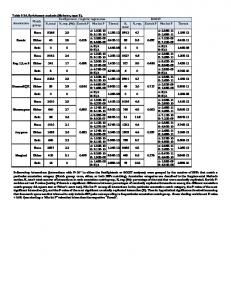
automatic processes to work entirely on their own. The dangers of letting the computer algorithms decide what is important or significant are well known (Flack and Chang, 1987; Freedman, 1983; Hauck, 1991). It is the analyst’s responsibility to carefully follow the results of each step of the variable selection process to determine if a better model may be indicated from the intermediates steps (as might frequently be the case from the first author’s experiences). Step 10. Array the “best” models within Steps 6-9 above in a table such as that found in Table 1, below. Note that in Table 1, only one model appears for each model due to space limitation reasons. In practice, one might have two or more models for each model-building process. Include fit indices such as the Hosmer-Lemeshow Goodness-Of-Fit (HL-GOF) as one (of many) criterion of fit. Make sure to check continuous variables for linearity in the logit (especially important if you get poor fit; see Hosmer and Lemeshow, 1989, page 89). If a parsimonious (i.e., simple) model is desired, the analyst may re-run the model-building process Steps 5-9 using the variables in Table 1 where: (1) all variables appear in every final model (e.g., in Table 1: Var3 and Var5), plus (2) variables that appear in a majority or higher of the models (e.g., in Table 1, if the variable appears in, say, two out of the three models: Var1, and Var2.) Table 1. Results of model-building process for outcome Model 1: Model 2: Model 3: Backward Forward Stepwise HL-GOF1=.73 HL-GOF1=.65 HL-GOF1=.23 Var1 Var1 Var2 Var2 Var3 Var3 Var3 Var4 Var5 Var5 Var5 1 HL-GOF=Hosmer-Lemeshow Goodness-of-Fit test Step 11. Compare all models in Step 10 on various fit indices (both numerical and graphical) and present to investigator as candidate models to choose from. For simplicity and space limitations, we use the HosmerLemeshow Goodness-of-Fit test (HL-GOF; Hosmer and Lemeshow, 1989). In practice, this test indicates a good model fit if its p-value ≥ .20 (closer to 1.0 is better.) The HL-GOF has two forms and has been shown to have sufficient power with sample sizes of about 400 or more. In Table 1, above, it can be seen that the best-fitting model is Model 1 with an HL-GOF of 0.73 and not far behind is Model 2 with an HL-GOF=0.65. However, though Model 3 has an HL-GOF of 0.23, it should not be discounted as a viable candidate model since its p-value is above the 0.20 standard cutoff. If Model 3 had a p-value of, say, less than 0.10, we might discount this model because of the poor fit or investigate its constituent variable properties to achieve a better fit.
METHODS & RESULTS Background of the CANCSP Data Data for the CANCSP were collected in 1996 and 1997 from 102 final clinic sites in California and from women 50
years of age or older receiving services at those sites (n=1,050 women.) To reduce survey costs, the data were first stratified into high and low density strata and then sites randomly chosen (as clusters) within those strata. Probability of selection weights were constructed to reflect the stratifiedclustered sampling design. Motivation Periodic mammography screening has a significant role in reducing mortality rates if utilized in the earlier stages. Even though one-time mammography use has increased over the past decade, repeat-screening mammography rates have not followed this trend. This is particularly true among lowincome immigrant populations who have a disproportionate number of breast cancer related deaths. While repeatscreening mammography in vulnerable populations has been indicated as a national priority, there is limited information available on factors associated with regular mammography screening adherence among uninsured, low income, immigrant populations. In fact, scant research has examined the relationship between the needs of uninsured immigrant women and health care system factors that have the potential to improve repeat-screening mammography. Cost and lack of insurance have repeatedly been cited as primary deterrents to regular breast cancer screening and as a reason for tumor stage difference at detection. However, simply having access to free services is not enough to eliminate barriers to regular mammography screening. This study explores individual, attitudinal, clinician, and health care system factors that may further explain repeat screening mammography adherence among uninsured immigrant women served by a state-wide no-cost-to-the-patient mammography screening program. For a more detailed discussion of barriers to repeat-screening mammography in the literature, see, for example, (Sabogal et al., 2003.) We next apply the methodology discussed in the Introduction, above. Variables in Steps 1-3 are exhibited in Appendix A. Step 1. The substantive variables chosen by the investigator are measures of (1) acculturation [ACULT4C; =less acculturation, 1=more acculturation], (2) access to healthcare [ACCHLTH; Range: 0-8; higher values mean more access], (3) decisional balance [DECBAL; -6 to 11; higher values mean more pros than cons], (4) intensity of the intervention [INTNSITY; Range: 3-15; higher values means more intense intervention], (5) doctor patient communication [MDPATCOM; Range: 3-7; higher values indicate more doctor/patient communication], and measures of whether the patient (6) got a mammogram because of a history of breast problems [R_H4B; 1=yes, 2=no], (7) imputed version of patient got mammogram because the doctor or nurse recommended it [R_H4FIMP: 1=yes, 2=no], (8) gets a Pap test following the recommended guidelines [R_M9PAPC; 1=yes, 0=no], and whether the clinic site has (9) an information or advice telephone line [A22G; 1=yes, 0=no] or (10) has in-reach services [A25; 1=yes, 0=no]. Step 2. Relevant demographic variables are included in this step (see Appendix A under the “Demographic vars” heading). Also secondary variables thought to be important in predicting regular mammography screening are whether the patient (11) took hormone pills [R_M4; 1=yes, 0=no], (12)
got their 1996 Pap test at the same time as their clinical breast exam (CBE) [R_M10R; 1=yes, 0=no], and the clinic site (13) percentage of White/Caucasian patients [A9B; Range: 0-84], (14) language fluency [A12_B; 1=≥50%, 0=