Rao, S.V.N., V. Sreenivasulu, S.M. Bhallamudi, B.S. Thanda- veswara, and K.P. Sudheer. 2004. Planning groundwater development in coastal aquifers.
c College of Urban and Environmental Sciences, Peking University, Beijing ..... modeling approach, Journal of Petroleum Science & Engineering 26(1): 273-282.
system; thus, jobs return to previous processing steps before leaving the system. ..... tasks are conducted by the maintenance technician MT1 in each machine ...
(recovered via the liquid collection and vapour recovery systems) to reactor grade and are referred .... and meaningful error messages keep the user on track. The user ... a dialog, so that input data can be entered or edited (Figure 3). Clicking ...
ROBERT FREDRIC JEFFERS find it satisfactory and recommend that it be ...... March 31. The adjudication performed by IDWR consists of a database of all water ...
Mar 18, 2013 - mental Modelling and Software, Jul 2012, Leipzig, Germany. ... Resources of a Limited Planet, Sixth Biennial Meeting, Leipzig, Germany.
Mar 18, 2013 - 2012 International Congress on Environmental Modelling and Software. Managing Resources of a Limited Planet, Sixth Biennial Meeting, ...
of Soil and Water Engineering, College of ... California, Davis CA 95616-8628, ... difficulties in solving design-operation problems in the field of engineering are ...
Jun 5, 2018 - Keywords: urban water resources; saving potentials; spatial allocation; ..... water demand; Qgreenbelt represents the urban green belt water.
We have proposed two alternates called Periodic. Boost and Spin Yield, and have ... of these different alternatives is needed to answer several open and crucial ..... 185.48 us. Table 3: Simulation parameters and values used in experiments.
Jan 31, 2017 - However, the constructed models are usually domain-specific in nature. The ..... Process. New Student Registration Process is a dynamic.
based hydrological and water resources forecasting models for real-world applications with best practices and a new forecasting framework. Free download until ...
Must the water networks be fail-proof or must they remain safe during a failure? What must water system managers try to achieve? The present paper introduces ...
activities are focused in the area of GIS and remote sensing on the .... District â 682 km2, Julfa District â 995 km2, Ordubad District â 972 km2, Sadarak. District ...
different simulation-based Approximate Dynamic Programming. (ADP)
approaches for the optimization of job sequencing and job releasing operations
in two ...
are used as local planning methods in sampling-based motion planning ... inputs are not guaranteed to give collision-free path segments. ... module, i.e., numerical integration of the differential equations which may ... tion II we provide a brief ov
PG(LLF,NLF,GLF,MARF,MERF,LCCF,QCCF). For further details, the implementation of this set of rules is shown in Ap- pendix A.1, written in Matlab notation ...
Aug 18, 2015 - Two-dimensional landslide dynamic simulation based on a velocity-weakening friction law. Abstract Surprisingly, hypermobility (high velocity ...
fresh water, of which about 0.3% is held in rivers, lakes, and ... Water shortages already exist in many regions, with more than one billion ... but also to human life and natural ecosystems (Pimentel et al. ... that receive low rainfall (less than 5
Jul 14, 2016 - located south east of Ilorin, Kwara State. The area has an open undulating land scope with occasional rocky outcrops in the north western part ...
architecture of the YAWL workflow management system with specific details on its service-oriented ..... lyon.fr/DIET/download/doc/UsersManualDiet2.4.pdf.
Aug 6, 2012 - regard to shared water resources, various types of games of- ... First classroom ap- plications of the ... also how to realize this solution in a situation where the best decision for ... been found to be beneficial for student learning
Implementation of a cloud-based microphysical precipitation model for data assimilation: ... seeks to merge different remotely sensed precipitation products,.
A Dynamic Flow Simulation Code Intercomparison based on the Revised .... Time-lapse seismic surface and down-hole measurements for monitoring CO2 ...
Feb 8, 2008 - The model is based on Powersim, a dynamic simulation software package capable of producing web-accessible, ..... of homes with drip irrigation will alter the homes with turf ..... Public Policy and Marketing 18 (2), 218e229.
Journal of Environmental Management 90 (2009) 471e482 www.elsevier.com/locate/jenvman
A dynamic simulation based water resources education tool Alison Williams a, Kevin Lansey b,*, James Washburne a,c b
a SAHRA Science and Technology Center, The University of Arizona, PO Box 210158b, Tucson, AZ 85721-0158, USA Department of Civil Engineering and Engineering Mechanics, The University of Arizona, Second and Palm Strs., Tucson, AZ 85721, USA c Department of Hydrology and Water Resources, The University of Arizona, Tucson, AZ 85721, USA
Received 23 October 2006; received in revised form 31 October 2007; accepted 30 November 2007 Available online 8 February 2008
Abstract Educational tools to assist the public in recognizing impacts of water policy in a realistic context are not generally available. This project developed systems with modeling-based educational decision support simulation tools to satisfy this need. The goal of this model is to teach undergraduate students and the general public about the implications of common water management alternatives so that they can better understand or become involved in water policy and make more knowledgeable personal or community decisions. The model is based on Powersim, a dynamic simulation software package capable of producing web-accessible, intuitive, graphic, userfriendly interfaces. Modules are included to represent residential, agricultural, industrial, and turf uses, as well as non-market values, water quality, reservoir, flow, and climate conditions. Supplementary materials emphasize important concepts and lead learners through the model, culminating in an open-ended water management project. The model is used in a University of Arizona undergraduate class and within the Arizona Master Watershed Stewards Program. Evaluation results demonstrated improved understanding of concepts and system interactions, fulfilling the project’s objectives. Ó 2007 Elsevier Ltd. All rights reserved. Keywords: Water Resources; Education; Modeling; Dynamic Simulation; Sustainability
1. Introduction The complexities of water resources systems can make it difficult for students and the public to understand the impacts of management decisions and the effects of conflicting uses, including their own, on the water balance. Water resources education opportunities are limited for adults who often have never learned more about water than the hydrologic cycle. A ‘big picture’ educational tool allows effective management and conservation alternatives to be considered and discussed. This tool enables adults to better understand water policy and resources in their community, thereby allowing them to participate in the development of equitable and sustainable water management as informed stakeholders. This article presents such a tool that is developed using dynamic simulation * Corresponding author. Tel.: þ1 520 621 2512. E-mail address: [email protected] (K. Lansey). 0301-4797/$ - see front matter Ó 2007 Elsevier Ltd. All rights reserved. doi:10.1016/j.jenvman.2007.11.005
software, has supporting documentation and tutorials and is user friendly and intuitive. Modeling has often been relegated to the academic and professional world, but, in the proper context, it can also be useful as an interactive and educational tool for non-technical individuals. ‘‘System dynamics can promote public participation by showing that our choices can affect the direction the future takes’’ (Stave, 2002, p. 165). System modeling enables the trial of policy options without having to accept the consequences (Shultz and Holbrook, 1999), as well as quick feedback from these options (Stave, 2002). Stave (2002, p. 144) states that, ‘‘For learning, models offer virtual worlds that allow people to discover for themselves how complex systems work through experimentation’’. Costanza and Ruth (1998, p. 186) conclude, ‘‘Thus, the modeling approach is not only dynamic with respect to the behavior of the system itself but also with respect to the learning process that is initiated among decision makers as they observe the system’s
472
A. Williams et al. / Journal of Environmental Management 90 (2009) 471e482
dynamics unfold’’. System dynamics modeling allows any model user to be a decision-maker for educational and exploratory purposes. System dynamics modeling has been used to highlight water management issues (Simonovic and Bender, 1996). It has recently been pioneered in public settings to help build policy or consensus for a policy (Stave, 2002, 2003; Simonovic and Bender, 1996; Costanza and Ruth, 1998; Passell et al., 2002). Tidwell et al. (2004) and Cockerill et al. (2005, 2006) applied system dynamics modeling with the goal of providing knowledge to the general public regarding the water issues in the Middle Rio Grande (NM). However, the use of modeling in strictly educational forms is limited, and this is the need the model herein was designed to fill. 2. Water resources education model objectives This model was developed as a tool to improve hydrologic literacy among college students and other adults. The model should also be accessible to high school students. The overarching objective of the model is to learn water resources principles and be capable of understanding their implications within a watershed. The three specific model goals are: 1. To provide users an understanding of critical hydrologic and water resource concepts, including consumptive use, population impacts on water demand, surface watere groundwater interactions, water use by sector, options for reclaimed water, safe yield, conservation alternatives, climate variability, and environmental effects of water use. 2. To present the system-wide implications of water management and policy alternatives. 3. To provide a setting for understanding conflicts in developing a comprehensive water plan and for conflict resolution. As an example, the concept of consumptive versus nonconsumptive uses is not well conveyed and understood by many. Without an understanding of this basic principle, it is difficult to make knowledgeable decisions on water use practices. To that end, goal 1 is achieved through a series of exercises that are applied by users to demonstrate significant water resources concepts. The model is then extended to a full water budget analysis and decision effects on the water balance and the components comprising the budget (goal 2). Finally, a multiple participant role playing exercise is posed with the goal of creating a sustainable system in terms of the water balance (goal 3). As an educational tool, the authors have strived to provide unbiased information to users in all exercises. For example, in the role playing task, participants are given goals for individual water use sectors but no guidance on maximizing those goals. These exercises are centered on a realistic generic system that allows concepts learned to be directly transferable to a specific region. Depending upon the learning exercise goals and participant’s knowledge, any of the three components can be used although it is preferable to begin with the introductory
material that will give users experience with the model and its interfaces. The following sections describe the model and the application system. 3. Water resources education model structure The overall model simulates the generic semi-arid region in Fig. 1 that contains various water supplies and demand sectors. The model has a time-step of 1 year with a simulation period of 25 years. The model consists of the following supplies: one river, one dammed river (reservoir), one aquifer, treated effluent, and options for imported or tribal water. Demand is based on an initial population of 675 000 with a population growth rate of 2.0%, which is one of the most important factors in the model. Agriculture demand is based on the following crop mix: cotton, alfalfa, lettuce, and wheat. The main focus of the model is on the water balance with only limited cost information. For example, farmer profit is included but conveyance and pumping costs are not. Each component of the model will be discussed in detail in the subsequent sections. 3.1. Supply The regional water supply system is composed of an uncontrolled river, a groundwater aquifer, a reservoir, imported water, tribal water rights, and treated effluent for potable uses. The combined central supply provides flow to four demand sectors: residential, agriculture, industrial, and non-residential turf. Each demand sector has unique paths to return flow to the system or to the atmosphere, including recharge, return to wastewater treatment plant (WWTP), and consumptive use (i.e., evaporation and plant growth). Some of these pathways return to the supply system, creating a positive feedback. Effluent treated for non-potable use is also recycled within the demand sector but it does not return to the central water supply because it can only be used for specific purposes. For simplicity, a priority order of water use is defined. The progression of water supplies that are used is; tribal water, imported water, reclaimed water for potable use, streamflow, reservoir diversions, and groundwater. Tribal and imported waters are purchased and must be used immediately. Given the cost of reclaimed water, we assume that it is also used immediately after treatment. Uncontrolled river flows are also used or lost while reservoirs and groundwater have the lowest priority since they can be stored over time. Detailed representations of each supply are described in the next subsections. 3.1.1. Supplementary external supplies Tribal water is a unique supply. It is intended to represent the allocation of water to Native American tribes that is common in the western US. We have assumed that some of these waters may be available for purchase. If the region cannot meet demand with initially available supplies, or if the aquifer is being overdrafted, the model allows the region to purchase and import a specific quantity of tribal water at a specific cost.
A. Williams et al. / Journal of Environmental Management 90 (2009) 471e482
473
RESERVOIR
INDUSTRIAL
Import/ Tribal
WATER SUPPLY
GW
Wastewater treatment plant
AGRICULTURE/ TURF
RESIDENTIAL
ENVIRONMENTAL/ RECREATIONAL AREA
RIVER
Flows into water supply or component Return flows to aquifer and river
GW – surface water flows Flow to wastewater plant Evaporation River
Fig. 1. Overview of components in the general water system.
If the water resources system is stressed enough to require this expensive acquisition, this supply will be used first. Imported water is also available to the region as an interbasin transfer or reallocation within the basin, such as Central Arizona Project water in Arizona or Central Valley Project water in California. Within the model, a specific water volume must be selected for purchase. If this volume is not needed to meet demand after full use of any purchased water, the remainder will be banked by recharging it to the aquifer. To convey the water to the basin, imported water will incur a supply expansion cost. The remaining artificial supply option is direct potable use of treated effluent. If this option is selected within the wastewater treatment operations, this designated supply will go directly into the ‘water supply’ for the region. The maximum quantity is based on the WWTP rules, discussed later, and a quantity up to this maximum, as needed, may enter the supply.
3.1.2. Natural supplies A set of simulation-period annual streamflow sequences is included in the model based on USGS historical data. Ten system configurations are available: a large or small river with wet, dry, or ‘average’ flow sequences, a user-defined flow sequence, or a user defined average flow that can be adjusted to a wet, dry, or ‘average’ sequence. The default flow condition of the model is the small river ‘average’ sequence. Streamflow is hydrologically connected to the aquifer, and the upstream reach may become losing if the groundwater level is drawn below a defined elevation. The region may divert a percentage
of the streamflow remaining after accounting for streamflow losses and minimum instream flow requirements. A reservoir on a second river receives inflows that are completely correlated and proportional to the free-flowing stream sequences (climate scenarios). The relationship between reservoir elevation and surface area is based on an Arizona reservoir. Precipitation and evaporation losses are based on Tucson-area meteorological data (AZMET, 2006) and the reservoir’s surface area. A minimum elevation for diversions and a maximum dam height are externally defined based on tabulated relationships from Salt River Project (AZ) data, and a downstream release requirement also must be satisfied. Water from the reservoir between the maximum and minimum levels may be diverted, as needed, after the minimum flow requirement is satisfied. If the minimum withdrawal is not completely diverted for use, the remainder is also released downstream and lost from the system. Groundwater is pumped only if the total of all other supplies cannot meet watershed demands. Groundwater availability is based on the initially defined aquifer storage that may be customized to the application. Groundwater extraction is allowed without limit to meet demands and is reported to the user. The goal of the role playing exercise goal is to eliminate aquifer overdraft. Aquifer recharge occurs directly from all demand sectors, as well as natural recharge from snowmelt, rainfall or channel recharge and direct or indirect recharge from wastewater treatment plant operations. Demand in excess of renewable supplies will be shown in the water budget as an overuse of renewable groundwater and result in a reduction in aquifer storage over time. Demand sector options to meet an overall balance are described in the next section.
474
A. Williams et al. / Journal of Environmental Management 90 (2009) 471e482
Fig. 2. Powersim water plan model main page.
3.2. Demand Four major demand sectors are included in the model: agriculture, industry, non-residential turf, and indoor and outdoor residential use. Demands increase with population growth and may be reduced by implementation of various conservation measures. 3.2.1. Agriculture sector Four common semi-arid region crops are assumed to be grown within the basin: alfalfa, upland cotton, durum wheat, and lettuce. Acreage for each of these crops can be varied within the model. An option to retire agriculture acreage, if selected, retires the same percentage of all crops with a onetime subsidy paid to the farmers. Crop water demand is estimated by its water use per acre and agriculture efficiency. Total agricultural water demand is the sum of the individual crop uses. The user may specify the percentage of agriculture acreage (except lettuce) to irrigate with treated effluent that is supplied by the WWTP and defined as agricultural effluent demand. The overall agricultural demand for new water is the total demand minus the effluent that is applied, that may be less than effluent demand if not enough is available. The ‘new’ water demand is taken from the water supply. A portion (16%) of the agricultural supply is assumed to recharge the aquifer while the majority is lost to consumptive use. The agriculture sector has direct economic returns based on an average crop yield per acre, price per unit, acreage cost and
costs per acre-foot for both ‘new’ water and effluent. Farmer profit is calculated from the profit for each crop and may be supplemented with land retirement payments. The default crop mix (and thus total water demand) may be overridden by user input of agricultural water demand. 3.2.2. Industrial sector Industrial use is calculated by multiplying the defined initial period demand by a linear industrial growth rate of 0.22%. Industrial effluent is sent to the wastewater treatment plant (68%), to the aquifer as incidental recharge (1.5%), and to the atmosphere as consumptive use (30.5%). No modeling options are provided in the industry use sector except to provide the initial industry demand. 3.2.3. Population The initial population is increased over time using the population growth rate. The number of households is computed by dividing the population by the persons per household. All of these variables may be modified. 3.2.4. Non-residential turf sector The non-residential turf sector consists of schools, public and private golf courses, and parks. This demand is calculated based on population density, acreage per sector, and water use per acre and summed across the four uses. Effluent can be used for any outdoor use by defining the percentage of any
A. Williams et al. / Journal of Environmental Management 90 (2009) 471e482
475
Fig. 3. Advanced user navigation page.
application using effluent. Turf demand for ‘new’ water is the difference between total turf demand and turf effluent use. Water cost is assessed based on the portions of ‘new’ water and effluent. A percentage of turf water demand (5%) is recharged to the aquifer as incidental recharge and the remainder is consumptive use. 3.2.5. Residential sector The residential demand sector is composed of indoor and outdoor components and is strongly based on population. Indoor use is the sum of toilet, shower, faucet, clothes washing machine, bathtub, dishwasher, and evaporative cooler uses. Each of these uses is computed as the product of the water use per action, the average actions per day per person, the average persons per house, and the current number of households. In addition, toilet use, shower use, and faucet use are broken into low-flow and traditional flow fixtures. Clothes washing use is broken into top-loader and front-loader (low water use) machines. The percentage of homes with frontloaders can be specified in model input. Potential water savings of switching all devices to low-flow is calculated, and a market penetration rate (that can be varied by the user) and efficiency rate for low-flow devices determine the actual retrofit water savings. Savings are subtracted from the sum of the other uses to obtain total residential indoor use. A percentage of water from all uses except for toilets may be used for gray water residential outdoor irrigation as selected by
the user. All remaining residential indoor demand is returned to wastewater treatment plants (i.e., no septic systems are considered). Residential indoor costs are a cost per unit for the ‘new’ water used, the costs of fixture replacements based on the market penetration rate of fixture retrofits, the number of fixtures per house, and the average cost of a retrofit or the cost associated with clothes washing machine investment (new homes) or replacement (existing homes). Residential outdoor use in the model consists of irrigation and pools. Turf and drip irrigation are modeled using turf area (acres) per household, water use per acre, and irrigation efficiencies. A default number of homes are assumed to have permanent fixed irrigated areas. Varying the percentage of homes with drip irrigation will alter the homes with turf as its complement. Like agriculture, a small percentage of the irrigation is recharged to the aquifer as incidental recharge. Irrigation water may be supplied by ‘new’ water from the water supply, effluent, gray water or rainwater harvesting. New irrigation water demand is the total demand minus supplies from the alternative sources that can be adjusted by the user. Pool use requires ‘new’ water for filter backwash, drainage, and evaporation replacement. The percentage of homes with pools may be varied by the user. Total residential outdoor demand is the sum of irrigation and pool demand. User costs for purchasing ‘new’ water and effluent are calculated. Residential indoor and outdoor uses are summed to compute the total residential use that is divided
476
A. Williams et al. / Journal of Environmental Management 90 (2009) 471e482
Fig. 4. Agriculture interface page. Slider bars are moved to modify the input value and results are plotted on the axes on the right side of the page. Numerical values are displayed for value during current model year. Initial values are shown here.
into ‘new’ water demand and alternative supplies. Water use per capita per day is also computed. 3.3. Wastewater treatment plant Residential and industrial sectors return water to the wastewater treatment plant through a collection system. The return flow is subjected to losses of 5% due to sludge disposal and evaporation. The remaining volume is available for reclaimed water use, aquifer recharge, or stream return. If effluent is required for stream return, a default of one half of all available inputs will return to the stream. Reclaimed water is then supplied for agriculture, turf, and residential outdoor irrigation users that can accept effluent based on user-defined percentages. Agriculture has first priority, followed by turf and residential outdoor. If indirect potable reclaimed use is allowed, aquifer recharge has the next priority. If direct treatment potable reclaimed use is allowed, effluent is first used as a water supply and, if the available volume is not required, the remainder will recharge to the aquifer. Any flow remaining after reclaimed uses (both potable and non-potable) will be returned to the stream. All water returned to the stream, as well as all streamflow in the downstream riparian area, will lose 25% to recharge and 30% to evapotranspiration. Expanding the effluent and reclaim system carries a fixed annual cost.
3.4. Environmental economics Monetary values associated with environmental benefits are included to demonstrate the competing interests in a regional water supply system. Based on downstream flow rates, values for floatboating, fishing, hiking, camping, and the preservation of "naturalness" are computed, and a value is also placed on streamflow reductions. These values are based on recreation demographics from Cordell et al. (1999) and averages of economic studies of ‘willingness to pay’ and ‘willingness to accept’. (These values will vary according to location, so no specific value ranges could be sourced for this model.) These studies can never represent the true environmental value, intrinsic or extrinsic, of streamflow, but this section is one attempt to represent an environmental point of view. 4. User interfaces The modules described above are modeled using Powersim Studio (Powersim, 2003). The resulting Powersim model is represented graphically with supporting equations that can be easily accessed, examined, and, if desired, changed. For user ease, Powersim includes a presentation mode in which user interfaces are constructed to display the essential input parameters and output variables. The main presentation
A. Williams et al. / Journal of Environmental Management 90 (2009) 471e482
477
Fig. 5. Residential interface page. Slider bars are moved to modify the input value and results are plotted on the axes on the right side of the page. Numerical values are displayed for value during current model year. Initial values are shown here.
mode interface page (Fig. 2) allows the user to select either a basic or advanced version as well as to view supplemental materials. The advanced version of the model contains an introductory navigation page (Fig. 3) that contains a brief model overview as well as links to all of the input and output pages. In all, the model contains nearly 400 model variables, approximately 25 decision variables that can be modified in each time-step, 30 user interface pages including about 75 control objects and a similar number of results objects (i.e., figures and tables). 4.1. Input pages The main demand sector interface pages are related to agriculture, turf, population, and residential sectors. Each page consists of user-controlled options and graphical and numerical results. Graphs on each page contain upstream and downstream streamflows and the aquifer level. These results show the effects of the user’s choices on the natural water system and on surface wateregroundwater interactions. The agriculture input page (Fig. 4) controls the acreage allotted to the four crops, the percentage of total acreage using reclaimed water, and the percentage of acreage that will be retired. The numerical values returned at the bottom of the page are the total agricultural water demand, ‘new’ and effluent demand, and the volume of recharged water. These numbers are valid for the current simulation year. Economic terms
that are presented are farmer profit, land retirement costs, and total farmer income. This page is designed to show the link between water use, farmer profit for alternative crops and the reductions in consumptive water use due to land retirement and from substituting reclaimed water. Exercises to demonstrate the water use interactions on each page have been developed and are described in the next section. Input from the turf page (not shown) is the percentage of each use that receives reclaimed water. Numerical results show total turf demand for each use, total turf demand for ‘new’ and effluent uses, turf recharge, and the yearly water cost. This page is designed to show that using reclaimed water is less costly for the turf ‘owner’ (i.e., private individual or governmental agency for parks). The residential page (Fig. 5) includes controls for various water conservation measures including the percentages of older homes with fixture retrofits, homes with front-loading washing machines, new homes with gray water technology, households with drip irrigation, households with rainwater harvesting systems, households with pools, and irrigation with reclaimed water hookups. This page displays numerical results for indoor, outdoor, and total residential demands that are broken into ‘new’ demand and alternative supply. Numerical values for the current year are also displayed for recharge, return flows to the system, cost of retrofits, and water cost. These values are all specified as a regional total and a per capita or per house use. This page is designed to demonstrate
478
A. Williams et al. / Journal of Environmental Management 90 (2009) 471e482
Fig. 6. Water budget output page.
the general effects of the set of water conservation actions on the water balance, specifically related to the different impacts of indoor and outdoor conservation. The final input page allows modification of the regional demographics by modifying population growth rate and persons per household (not shown). It displays population and the number of households with plots of streamflow, aquifer storage and residential and turf demands. These decisions are designed to show the sensitivity of population growth on future demand trends with emphasis on outdoor consumptive uses. After defining all parameters and desired measures to be implemented, an input summary page is available so the user can see all of their decisions in one location. Input can also be modified from this page. 4.2. Output pages The water budget interface (Fig. 6) displays numerical results including ‘new’ water demand, reclaimed water demand, return flows to system, and recharge for the four demand sectors. These results summarize the impact that each sector has on total and consumptive use. The available water and actual use from the six supplies are also listed to show supplies that are over- or under-utilized. The streamflow graph is presented with an aquifer balance as opposed to aquifer volume to focus on aquifer overdraft. Within the model, demand can never exceed supply because groundwater will be used to meet all demands even if the aquifer is overdrafted. The water
budget page therefore provides guidance on selecting general options that can be taken to make the system sustainable. A result that may be perceived as equally important as the water balance is system costs. A second interface itemizes and plots the supply costs incurred for the selected plan and an environment results page displays the environmental economic values and an explanation of the process of environmental economic valuation. This result is designed to demonstrate that water in the river is not beneficial simply to supplement supply, but also for recreation, riparian, aesthetic, and intrinsic benefits. Ancillary results are also provided that are not linked directly to the task of developing a water balance. The riparian area page shows the consequences of various decisions on the downstream riparian habitat. Details on riparian zone processes that affect the flow in the riparian area and downstream streamflow are also summarized. A reservoir page shows the temporal history of reservoir storage to show the effects of decisions on its operations. 4.3. Advanced input and customization pages Beyond the basic model pages, the model contains three control interfaces for customizing the region, selecting certain supply and treatment options and specifying the flow sequence. On the customization page, the user can modify the initial aquifer volume, natural recharge rate, initial population, industrial water demand, and agriculture water demand. The industrial and agriculture water demands override the model’s regional default values. The other inputs change initial model
A. Williams et al. / Journal of Environmental Management 90 (2009) 471e482
479
Fig. 7. Control page that permits input of various global decisions and settings.
parameters. On the supply and treatment controls page (Fig. 7), the user may select from a variety of operational procedures including: the amount of water to import and whether or not to treat it, the amount of tribal water to purchase and at what rate, whether or not to have a reservoir, the reservoir diversion rate, whether or not to use reclaimed water for potable use, and whether or not to require effluent for the stream. Each of these options has consequences discussed in the module descriptions, often involving cost. The final input interface page (not shown) consists of flow selection. The user can select 1 of 10 flow sequences described earlier, define an instream flow requirement, and select how much of the remaining flow should be diverted for use. 4.4. Supporting material The impact of climate on a system’s water balance can be significant. A climate page and associated climate diagram (not shown) are included to explain the variations in the annual flow sequences available. Additional supporting material for running the model and a glossary of terminology definitions are given on additional pages.
Project, and Control Case Studies. In addition, a User’s Manual was developed as an instructor aid or for those teaching themselves. Although this model was not developed in a participatory process, it was designed to open discussion regarding water resources, with many questions and activities left open-ended. 5.1. Introductory questions The introductory questions isolate individual components of the water supply system to simplify the system and focus the student on a specific process. Six question sets deal with Turf, Agriculture, Residential, Population, the Water Budget, and Riparian Area. Each of the first four sets isolates a limited number of variables to show the user how to isolate the effect of a single option on different results, and the last two sets deal with overall system results. Each group of questions addresses a hydrologic or water resource concept. For example, the objectives for the first question set that are related to turf irrigation are: To identify the benefits of using reclaimed water for non-potable uses, to discover the price difference between ‘new’ and reclaimed water, and to identify the water demand for the turf sector. Table 1 summarizes the question set and concept relationships and Fig. 8 illustrates an exercise related to turf irrigation.
5. Supplementary materials 5.2. Water management project To achieve the noted goals, a set of supplementary materials have been prepared that emphasize certain concepts. The activities include Introductory Model Questions, a Water Management
Once the students have familiarized themselves with the introductory concepts and their effects, the next step is to use
A. Williams et al. / Journal of Environmental Management 90 (2009) 471e482
480
Table 1 Relationship between introductory questions and project goals Question
Topic
Concept(s) from goal 1
One
Turf
Two
Residential
Three
Agriculture
Four
Population
Five Six
Water budget Riparian area
Reclaimed water, water demand by sector (turf) Consumptive use, conservation alternatives, water demand by sector (residential) Water demand by sector (agriculture and residential), conservation alternatives Effects of population growth, surface and groundwater interactions Water demand by sector (all), safe yield Environmental effects
look at the students’ water management plans in light of different climate scenarios. The students are asked to see if their plan still meets safe yield with different levels of streamflow, and if not, how to address this problem. The second case study asks the user to vary the supply and wastewater treatment controls to see the effects of those changes on the system’s water balance and, if safe yield can be achieved at an acceptable financial and environmental cost. This case study’s main purpose is to differentiate between implications of supply-side and demand-side management. 6. Implementation results
this information to develop a water management plan. Students are assigned to groups of four to develop a plan that will meet safe yield (i.e., maintaining groundwater extraction less than or equal to recharge) throughout the 25 year simulation. Each of the students represents a different interest; farmer, developer, environmentalist, or negotiator. The group must identify a plan that is acceptable to the entire group while considering the effects on individual roles and the entire water system. Finally, they must consider if their plan can be realistically implemented. This is an open-ended exercise with no right or wrong answers and is designed to bring out differing viewpoints and discussion. 5.3. Control case studies The final exercise consists of two supplemental case studies. The first case study, climate variability, requires a new
A preliminary implementation and evaluation was completed in the Spring 2005 semester of the University of Arizona course, Hydrology and Water Resources (HWR) 203 entitled Arizona Water Issues. This implementation used three class periods totaling 3 h and 45 min and involved 55, primarily lower division, students. After that offering, the model and supplementary materials were refined for implementation in Fall 2005. The second classroom implementation used four class periods totaling 5 h with 45 similar students. Finally, one community outreach implementation took place for a 4-h session of Pima County Master Watershed Stewards (MWS) with 12 students. MWS is a volunteer program that caters primarily to adults who are interested in learning about water and making a difference in their watershed. The students are generally much more mature with a broader life experience than those in the undergraduate classes. In both settings, after
1) Turf: A. Fill in the first column of the following chart with the default, initial year values (Note: default values are the input numbers in the model when it is opened or reset, and initial year values are the values before running the simulation, i.e. 1/1/2005). Then change private golf courses, parks, and schools to 50% reclaim and fill in the second column. Default Values 50% Reclaim Turf New Demand kafy kafy Yearly Water Cost $ $ [These units are somewhat odd but needed when discussing large water volumes. An acrefoot or af is a water volume and is equivalent to one acre of land covered with 1 foot of water (acre * foot). An acre-ft/year is the rate at which water is used or a volume per time. A kafy is1000 acre-ft per year. An acre-foot of water is quite large. It is equal to 325,000 gallons or the annual in door and outdoor use of 1 to 2 urban households. One acre is 43,560 square feet so one acre-ft is 43,560 cubic feet (ft3). An average tractor trailer (without the cab) is about 8 ft. wide, 10 ft. high and 48 ft. long or 3840 ft3 (=8*10*48) so 1 acre-ft is equivalent to over 11 tractor trailers filled with water (11.35 to be exact).] Based on the table above,how much new water can be saved for other uses if at least 50 % of turf uses reclaimed water?___________ kafy Is reclaimed water cheaper or more expensive than new water? (In other words,does increasing reclaimed water increase or decrease yearly water cost?) B. How much water does a single 18-hole private golf course use? (Use the Water Demand and Number of holes in the Private Golf Course column. You need to do some math.) _________afy Fig. 8. Introductory questions related to turf irrigation.
A. Williams et al. / Journal of Environmental Management 90 (2009) 471e482
481
Table 2 Comparison of student concept before (pre-test) and after understanding model exercises (post-test) Topics
Consumptive use Population impacts on water demand Surface watereground water interactions Water use by sector Options for reclaimed water Safe yield Conservation alternatives Climate variability Environmental effects of water use a
1 ¼ No understanding, 3 ¼ average understanding, and 5 ¼ exceptional understanding.
an introduction by the instructor, students completed the activities in small groups.
6.1. University of Arizona HWR 203 Fall 2005 To evaluate the model and materials, self-assessment and actual knowledge pre- and post-tests were developed and given to sample sizes of 28 and 26 for the pre- and post-test, respectively, with 20 students taking both tests. The overall sample had increases between 9% and 39% on self-assessment of nine important concepts, while the subsample that took both the pre- and post-tests had statistically significant increases in every topic (Table 2), demonstrating student learning. Actual knowledge assessment multiple-choice questions also produced positive results. The percentage of students identifying gaining and losing reaches as the connection between surface and groundwater increased from 14.3% to 65.4% compared to those who knew they were connected but did not know how, which decreased from 46.4% to 3.8%. The percent identifying water not returned to the system as the correct definition for consumptive use increased from 28.6% to 84.0% and incorrect responses also declined significantly. A majority (80.8%) of respondents knew the correct legal definition of safe yield up from 40.7% in the pre-test. The question addressing current or potential uses of reclaimed water did not result in any statistically significant improvement. When asked to identify conservation alternatives, fixture retrofits were identified by 84.6%, up from 48.1% on the pre-test, and the percentage of students who identified drip system irrigation increased from 74.1% to 88.5%. People answering that climate variability, which was not fully addressed due to time constraints, always affects the water budget increasing from 53.6% to 69.2%. Most of the students (96.2%) on the post-test identified ‘to maintain riparian health’ as an answer for ‘why is it good to have sufficient flow in a river,’ up from 60.7%. A paired t-test on the subsample shows statistical significance for each statement agreement category except for the first (Table 3). The second and third statements are specific
goals for the model and intended to measure the ‘big picture’ education of the project by asking if students agree that they understand some implications of water management alternatives, conflicts between users, and ways to solve them. Both of these statements show positive results. The fourth and fifth statements were assessments of what behavioral changes students might make outside the classroom and are not directly related to the project goals. The results indicate that students learned the consequences of their actions, but do not prove that their behavior will change. In addition to the positive results for all previous evaluation components, 84.6% of students felt the model improved their understanding of class concepts, and 73% of students felt the model had above-average effectiveness. Most of the students (96.2%) indicated the user-friendliness of the model was between fair and extreme, with a mean around very user-friendly. Instructor experience and the comments section indicate that class attendance and quality of instruction are very important to model success. An instructor must make a serious commitment to become familiar with the model and to require attendance and participation from all students. Table 3 University of Arizona Fall 2005 HWR 203 statement agreement before (pretest) and after model exercises (post-test) (n ¼ 20) Statements
There is a water problem in Arizona I understand some implications of water management alternatives I understand some conflicts between water users and can think of options to resolve them I think I could effectively participate in a political process related to water issues I do now or soon plan to practice water conservation at home
Pre-test
Post-test
Paired t-test (one-tail)
Meana
Meana
P
4.25
4.16
0.358116
2.80
3.74
0.000106
3.30
3.90
0.005081
2.68
3.10
0.020931
3.50
3.90
0.036195
a Average agreement with statements. 1 ¼ Strongly disagree, 2 ¼ disagree, 3 ¼ neutral, 4 ¼ agree, and 5 ¼ strongly agree.
482
A. Williams et al. / Journal of Environmental Management 90 (2009) 471e482
6.2. Fall 2005: Master Watershed Stewards This class spends 10 weeks focusing on a variety of water resource concepts, so the biggest concern was to see if the model could effectively bring all the information together and communicate ‘big picture’ management alternative concepts. It was assumed and verified through pre-evaluation that the class had a good understanding of basic hydrologic concepts. However, statistically significant increases ( p < 0.05) were still seen in five of the nine concepts; population impacts, surface wateregroundwater interactions, water use by sector, safe yield, and conservation alternatives (Table 2). Knowledge assessments also showed significant improvement in three of those categories. The percentage of students correctly selecting gaining and losing reaches as the connection between surface and groundwater increased from 80% to 100%, and the percent correctly defining safe yield rose from 77.8% to 100%. In addition, the correct definition of consumptive use was selected by 91.2% on the post-test, up from 45% on the pre-test. Owing to the overwhelmingly high responses on the pre-test statement agreement section, there were no statistically significant increases from the pretest to the post-test, although there were increases in every category. Despite the fact that some of this project was a repetition of class material, 92% felt the model improved their understanding of class concepts and 92% also rated the overall effectiveness as above-average. In addition one person wrote in the comment section that they most enjoyed ‘‘experiencing the big, complicated picture of water needs, use, and conservation,’’ a very good summation of the overall project goal. 7. Conclusions and future work The main goal of this work was to develop ‘big picture’ water-system educational tools that are useful to a wide and diverse audience of college students and other adults. An example of the success of this project was observed even with students who were apathetic and had low attendance. Thus, the success of the model in the Fall 2005 HWR 203 class as shown by evaluation results demonstrate that not only does the model meet the overall ‘big picture’ goal, but it also provides an alternative learning technique that can engage a variety of users who may not respond well to traditional teaching formats. Therefore, the benefits of the model are twofold in that it helps provide hydrologic literacy and may connect with an audience that may otherwise have been lost. Several opportunities to extend the use of the model are seen. The most significant is to transfer the model to the internet to facilitate distribution. In addition, enhanced interfaces with graphics and inquiry tools can help decrease dependence on instructor-led use and may increase user enjoyment which was one of the lower scores on the evaluations. Materials for
use in high school settings would not need to differ greatly from those produced for the university and outreach programs, but materials for lower grades could be created with minimal time commitment from someone familiar with educational standards. Acknowledgements The authors acknowledge and appreciate the input and support of Candice Rupprecht, Paul Wilson, Steve Stewart, Robert Emmanuel, Michael Crimmins, Derya Sumer, and Gunhui Chung. This work was supported by the University of Arizona, Technology and Research Initiative Fund (TRIF), Water Sustainability Program and by SAHRA (Sustainability of semiArid Hydrology and Riparian Areas) under the STC Program of the National Science Foundation, Agreement No. EAR9876800. Any opinions, findings, and conclusions or recommendations expressed in this material are those of the author(s) and do not necessarily reflect the views of SAHRA or of the National Science Foundation. References AZMET, The Arizona Meterological Network, 2006. Tucson Station Data Files. http://ag.arizona.edu/azmet/data/0104et.txt (accessed 10.06). Cockerill, K., Tidwell, V., Passell, H., 2005. Assessing public perceptions of computer-based models. Environmental Management 34 (5), 609e619. Cockerill, K., Passell, H., Tidwell, V., 2006. Cooperative modeling: building bridges between science and the public. Journal of the American Water Resources Association 42 (2), 457e471. Cordell, H.K., Betz, C., Bowker, J.M., English, Donald B.K., Mou, S.H., Bergstrom, J.C., Teasley, R.J., Tarrant, M.A., Loomis, J., 1999. Outdoor Recreation in American Life: a National Assessment of Demand and Supply Trends. Sagamore Publishing, Champaign, IL, xii, 449 pp. Costanza, R., Ruth, M., 1998. Using dynamic modeling to scope environmental problems and build consensus. Journal of Environmental Management 22 (2), 183e195. Passell, H.D., Tidwell, V.C., Webb, E., 2002. Cooperative modeling: an approach for community-based water resource management. Southwest Hydrology 1 (4), 26. Powersim Software AS, 2003. Powersim Studio 2003 User’s Guide. http:// www.powersim.com. Bergen, Norway (accessed 10.06). Shultz II, C.J., Holbrook, M., 1999. Marketing and the tragedy of the commons: a synthesis, commentary, and analysis for action. Journal of Public Policy and Marketing 18 (2), 218e229. Simonovic, S.P., Bender, M.J., 1996. Collaborative planning-support system: an approach for determining evaluation criteria. Journal of Hydrology 177, 237e251. Stave, K.A., 2002. Using system dynamics to improve public participation in environmental decisions. System Dynamics Review 18 (2), 139e167. Stave, K.A., 2003. A system dynamics model to facilitate public understanding of water management options in Las Vegas, Nevada. Journal of Environmental Management 67, 303e313. Tidwell, V.C., Passell, H.D., Conrad, S.H., Thomas, R.P., 2004. System dynamics modeling for community-based water planning: application to the middle Rio Grande. Aquatic Sciences 66, 357e372.