GC-Tree: A Fast Online Algorithm for Mining

GC-Tree: A Fast Online Algorithm for Mining Frequent Closed Itemsets Junbo Chen, ShanPing Li Department of Computer Science, ZheJiang University Dorm 10, 5035, Zhejiang University YuQuan Campus, Hangzhou City, Zhejiang Province, China [email protected] [email protected]

Abstract. Frequent closed itemsets is a complete and condensed representaion for all the frequent itemsets, and it’s important to generate non-redundant association rules. It has been studied extensively in data mining research, but most of them are done based on traditional transaction database environment and thus have performance issue under data stream environment. In this paper, a novel approach is proposed to mining closed frequent itemsets over data streams. It is an online algorithm which update frequent closed itemsets incrementally, and can output the current closed frequent itemsets in real time based on users specified thresholds. The experimental evaluation shows that our proposed method is both time and space efficient, compared with the state of art online frequent closed itemsets algorithm FCI-Stream [3].

1 INTRODUCTION Frequent closed itemsets is a complete and condensed representation for all the frequent itemsets. Therefor, the study of the Frequent closed itemsets has arisen a lot of interest in the data mining community. Extensive researches have been carried out in this area, in the following they are split to four categories : Both A-Close [12] and TITANIC [8] exploit a level-wise process to discover closed itemsets through a breadth-first search strategy. In each iteration, they try to search for candidates of MGs (Minimum Generators) with the help of search space pruning technique, and then verify them. Finally the MGs are used to generate all the closed itesmsets . Usually these algorithms are required to scan the whole dataset many times. For CLOSET [13] and CLOSET+ [6]. With the help of high compact data structure FP-Tree, they try to project the global extraction context to some smaller sub-contexts, and then apply FCI mining process recursively on these sub-context. Better performance can be achieved than the adoption of A-close and TITANIC algorithms. CHARM [7] and DCI-Closed [4] exploit hybrid techniques which try to use the properties of both previous mentioned techniques. Due to a data structure called ITTree, CHARM simultaneously explores both the closed itemset space and transaction space, with the depth-first search strategy, and generates one candidate each time, then with tidset intersection and subsumption checking, it will see whether the candidate is closed. DCI-Closed could be considered as an improvement of CHARM.

2

GC-Tree: A Fast Online Algorithm for Mining Frequent Closed Itemsets

FCI Stream [3] is an online algorithm which performs the closure checking over a data stream sliding window. It uses a in memory data structure called DIU-tree to store all the Closed Itemsets discovered so far. With a specific search space pruning technique, it tries to perform the time consuming closure checking operation only when it’s really needed. Among all the algorithms, DCI-Tree has the best performance. Inspired by this algorithm, in this paper, we try to adapt it as an online algorithm under data stream sliding window environment, called GC-Tree.This algorithm is named after the in memory data structure it used, which is also called GC-Tree. The rest of this paper is organized as follows. Section 2 formally defines the concept of closed itemsets, describes the notations to be used throughout the paper and introduces related works. Section 3 presents our proposed GC-Tree algorithm. The performance evaluation is depicted in Section 4. Finally, comes conclusion of this paper, Section 5.

2 PROBLEM DEFINITION Let I = {i1, i2 , ..., in } be a set of items, D = {t1 , t2 , ..., tn , ...} be a set of infinite stream of transactions, and S = {tx0 , tx1 , . . . , txM } be a sliding window of D which contains the recent M transactions. A subset I ⊆ I is called an itemset. Each transaction t ∈ D is a set of items in I. There’s an unique transactionid for every t. Given a set of transactions T ⊆ D, it can be represented by a tid list, and the support of an itemset I in T is the percentage of transactions that contain I. The concept of a closed itemset is based on the two following functions: f (T ) = {i ∈ I | ∀t ∈ T, i ∈ t} g(I) = {t ∈ D | ∀i ∈ I, i ∈ t} Definition 1 An itemset X is said to be closed if and only if C(I) = f (g(I)) = f ◦ g(I) = I where the composite function C = f ◦ g is called a Galois operator or a closure operator. As a closure operator, C have the following properties: Property 1 C(X) ⊇ X Property 2 Y ⊆ X ⇒ C(Y ) ⊆ C(X) Property 3 C(C(X)) = C(X) The number of transactions in the dataset including an itemset I is defined as the support of I, denoted as supp(I). Mining all the frequent closed itemsets from the current sliding window of data stream D requires to discover all the closed itemsets which have higher support than a given threshold min supp in the sliding window. The closure operator, C defines a set of equivalence classes. All elements belong to the same equivalence class share the same closed itemset. Our algorithms tries to find exactly one generator in every equivalence class, then calculates the closure of them. There’re 2 popular lemmas which are wildly exploited: Lemma 1 Given two itemsets X and Y , if X ⊂ Y and supp(X) = supp(Y ), then C(X) = C(Y ). Lemma 2 Given an itemset X and an item i, if g(X) ⊆ g(i) ⇒ i ∈ c(X).

GC-Tree: A Fast Online Algorithm for Mining Frequent Closed Itemsets

3

3 THE GC-TREE ALGORITHM 3.1 Algorithm Overview Our algorithm is inspired by ’DCI Closed’ algorithm [4], It exploits a total lexicographic order relation ≺ among all the itemsets of the search space 1 . The usage of a closure climbing technique to obtain closure generators on the basis of the total lexicographic order, can efficiently detect the duplicate generators in the same equivalence class. In this paper, we propose an algorithm which can work under the data stream sliding window environment. This algorithm uses an in memory data structure called GC-Tree (Generator and frequent Closed itemsets Tree) to store all the frequent closed itemsets in the current sliding window. Each element in The GC-Tree has the following format: < gen, eitem, clo >2 . Where gen is the closure generator, eitem is the extension item with which gen used to extend another closed itemset3 , clo is the corresponding closed itemset4 . We also define two functions on the gen, preset(gen) and posset(gen) which are defined as: Definition 2 Let gen = Y ∪ i be a generator of a closed itemset where Y is a closed itemset and i ∈ / Y . preset(gen) is defined as {j ≺ i|j ∈ / gen}. posset(gen) is defined as {j ∈ I|j ∈ / preset(gen) and j ∈ / C(gen)}. Definition 2 along with Definition3, Theorem 1 and Lemma3 provided by Claudio Lucchese et al [4] are the base of our GC-Tree algorithm: Definition 3 A generator X = Y ∪ i, where Y is a closed itemset and i ∈ / Y , is said to be order preserving one iff i ≺ (C(X) − X). Theorem 1 For each closed itemset Y 6= C(∅), there exists one and only one sequence of n(n ≥ 1) items i0 ≺ i1 ≺ . . . ≺ in−1 such that {gen0 , gen1 , . . . , genn−1 } = {Y0 ∪ i0 , Y1 ∪ i1 , . . . , Yn−1 ∪ in−1 } where the various geni are order preserving generators, with Y0 = C(∅), Yj+1 = C(Yj ∪ ij )∀j ∈ [0, n − 1] and Y = Yn . Lemma 3 Let gen = Y ∪ i be a generator of a closed itemset where Y is a closed itemset and i ∈ / Y . gen is not order preserving iff ∃j ∈ preset(gen), such that g(gen) ⊆ g(j). GC-Tree is lexicographically ordered, for each closed itemset, there exists a path in GC-Tree from the root. All the elements in this path compose the order preserving generator sequence {gen0 , gen1 , . . . , genn−1 } mentioned in Theorem 1. It has the following properties : Property 4 Let Np < gen, clo > be parent node of Nc < gen, clo > in GC-Tree, Then we have: (1) Nc .gen = Np .clo ∪ j, j ∈ Np .pos and gen is order preserving in every Node. (2) Nc .gen ⊃ Np .gen. (3) Nc .clo ⊃ Np .clo. (4) posset(Nc .gen) ⊂ posset(Np .gen) Property 5 Every Frequent Closed Itemset in the current sliding window can be 1

2

3 4

This lexicographic order is induced by an order relation between single item literals, according to which each k-itemset I can be considered as a sorted set of k distinct items {i0 , i1 , ..., ik }. For the concision of representation, we omit the links between the parents and children, and the support of the closed itemsets eitem is the item i in Definition 2 The GC-Tree Node may be written in the compact way in the rest of this paper: < gen, clo >

4

GC-Tree: A Fast Online Algorithm for Mining Frequent Closed Itemsets

found in the GC-Tree, the path from the root to the specific FCI composes the sequence {gen0 , gen1 , . . . , genn−1 } in Theorem 1 Property 6 Let Nr < gen, clo > be the root in the GC-Tree, then we have Nr .gen = ∅ , Nr .clo = C(∅), preset(Nr .gen)=∅ and posset(Nr .gen)=I − C(∅)

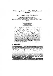
Fig. 1: GC-Tree

When a transaction arrives or leaves the current sliding window, the algorithm update GC-Tree incrementally. Figure 1 illustrates the GC-Tree when the data stream {A, AB, CD, ABCD} arrives. 3.2 Add a Transaction to the Sliding Window In this section, we discuss how to maintain the GC-Tree when a new transaction arrives. Let t be the arrived transaction, T1 be the set of transaction in the sliding window before t comes, T2 be the set of transaction in the sliding window after t comes, then we have: T2 = T1 ∪ t Lemma 4 Let CT1 be all the closed closed itemsets in T1 , and CT2 be all the closed closed itemsets in T2 , then we have: CT1 ⊆ CT2 Proof: ∀c ∈ CT1 . if c ∈ / t, then, g(c)T2 = g(c)T1 ⇒ f (g(c)T2 ) = f (g(c)T1 ) = c ⇒ c is closed. If c ∈ t, then, g(c)T2 = g(c)T1 ∪ t ⇒ f (g(c)T2 ) = f (g(c)T1 ) ∩ t = c ∩ t = c ⇒ c is closed. According to Lemma 4, when a new transaction is added to the sliding window, the only action we should concern is to add new nodes(closed itemsets) into FCI-Tree. 3.2.1 The conditions to add new closed itemsets Lemma 5 Let Y * t ⇒ C(Y )T 2 = C(Y )T 1 Proof: g(Y )T2 = g(Y )T1 ⇒ C(Y )T 2 = f (g(Y )T2 ) = f (g(Y )T1 ) = C(Y )T1 . According to Lemma 5, If Y * t, Y will remain closed/un-closed in T2 as in T1. So, we simply omit this situation. Lemma 6 Let Y ⊆ t, t ∈ T1 ⇒ C(Y )T 2 = C(Y )T 1 According to Lemma 6, If Y * t, and t ∈ T1 Y will remain closed/un-closed in T2 as in T1. So, we simply omit this situation, too. 3.2.2 How to add new closed itemsets to GC-Tree First, we give the pseudo-code algorithm in Table 1, then we explain how it works.

GC-Tree: A Fast Online Algorithm for Mining Frequent Closed Itemsets

5

Table 1: GC-Tree−Addition 1: procedure Add(t, curr) 2: if(t ∈ T1 ) 3: for all Y ∈ t, Y is closed itemset: s(Y)++; 4: return; 5: else 6: if(curr.gen * t) return; 7: newclo ←− curr.clo ∩t 8: if(newclo = curr.clo ) 9: s(curr.clo)++; 10: for all (i ∈ posset∗ (curr)) 11: checkChild(curr.clo ∪ i, curr, t) 12: else 13: m ←− min≺ {curr.clo − newclo} 14: newnode ←− 15: s(newnode.clo) ←− s(curent.clo); 16: for all (child of curr node) 17: if(child.eitem ∈ preset(newnode)) 18: moveChild(child, curr, new-node); 19: else 20: child.gen ←− newclo ∪ child.eitem; 21: addChild(curr, new-node); 22: curr.clo ←− newclo; 23: for all (i ∈ posset∗ (curr)) 24: checkChild(curr.clo ∪ i, curr, t)

In Table 1, preset(node) is defined as the preset of node.gen, posset(node) is the posset of node.gen, posset∗ (gen) is defined as posset(gen) ∩ t, moveChild(child,oldparent,new-parent) detaches child from old-parent and add it as a child of new-parent, checkChild(curr.clo ∪ i, curr, t) searches the children of curr node: if any of them have gen = curr.clo ∪ i, the algorithm invokes Add() recursively; if there’s no such child found, the algorithm invokes closureCheck(curr, t) function5 , and closureCheck() is defined in Table 2. According to Lemma 6, it’s unnecessary to perform any operation if t ∈ T1 except to increase the supports, see Table 1, line 2-4. Lemma 7 Let CT1 be all the closed closed itemsets in T1 , and CT2 be all the closed closed itemsets in T2 , ∀ci ∈ (CT2 − CT1 ), we have: ci ⊆ t Proof: if ∃cj * t, then we have, g(cj )T2 = g(cj )T1 ⇒ C(cj )T2 = C(cj )T1 , which means cj will remain closed/un-closed in T2 as in T1, so that cj ∈ / (CT2 − CT1 ). According to Lemma 7, we have, gen * t ⇒ C(gen) * t ⇒ C(gen)T2 = C(gen)T1 , and notice that if gen * t, then for any offspring of the current node, we have gen * t, that means there should be no new closed itemset in the current node and its sub-tree, see Table 1, line 6. 5

Similar to the function closureCheck() in DCI-Closed, devised by Claudio Lucchese et al [4]

6

GC-Tree: A Fast Online Algorithm for Mining Frequent Closed Itemsets Table 2: GC-Tree−Closure Checking

1: procedure closureCheck(parent, item) 2: gen ←− parent.clo ∪ item 3: if(is dup(gen) = f alse) 4: newclo ←− gen; 5: for all j ∈ posset∗ (parent.gen), j  itemm, g(gen) ∈ g(j) 6: newclo ←− newclo ∪j 7: new-node ←− < gen, newclo>; 8: addChild(parrent, new-node); 9: for all k, k ∈ posset∗ (gen) 10: closureCheck(this, k)

Lemma 8 For any node n in the GC-Tree, if n.gen ⊆ t, we have: C(n.gen)T2 = C(n.gen)T1 ∩ t Proof: C(n.gen)T2 = f (g(n.gen)T2 ) = f (g(n.gen)T1 ∪ t) = C(n.gen)T1 ∩ t. According to Lemma 8, we have: if curr.gen ⊆ t and curr.clo = curr.clo ∩ t, then the closed itemset in the current node remains closed, so we leave the current node alone and checking it’s children. See Table 1, line 8-11. Lemma 9 For any node n in the GC-Tree, if n.gen ⊆ t and C(n.gen)T2 6= C(n.gen)T1 ∩ t, then ∃i ∈ I which makes gen∗ = C(n.gen)T2 ∪i order preserving and C(n.gen∗ )T2 = C(n.gen)T1 Proof: First, we prove gen∗ is order preserving: According to Lemma 8, it’s easy to see C(n.gen)T1 ⊇ C(n.gen)T2 . Let i = min≺ {C(n.gen)T1 − C(n.gen)T2 }, obviously, gen∗ = C(n.gen)T2 ∪ i is order preserving. Second, we prove C(n.gen∗ )T2 = C(n.gen)T1 : C(n.gen∗ )T2 = f (g(n.gen∗ )T2 ) (1) = f (g(C(n.gen)T2 ∪ i)T2 ) (2) = f (g(C(n.gen)T2 ∪ i)T1 ) (3) = C(C(n.gen)T1 ) (4) = C(n.gen)T1 (5) Equation (3) holds because i ∈ / t (see Lemma 8), equation (4) holds because in T1 , C(n.gen)T2 ∪ i and C(n.gen)T1 belongs to the same equivalence class. According to Lemma 9, if the clo of the current node is changed after t arrives, the new clo = C(gen)T2 is simply C(gen)T1 ∩ t, and a new node < gen∗ , C(gen)T1 > is required as a child of the current node. To make sure the children of current node are order preserving in the updated GC-Tree: if j is not in the preset of the new node, we should move them from the current node to the new node as children; else, we set the child.gen as C(gen)T2 ∪ j 6 . See Table 1, line 12-24. 6

This is acceptable because it’s easy to proof if j ∈ / t, then the closure of the new generator equals to the closure of the old generator, if j ∈ t, then the recursive checking would find the closure of the new generator, pushing down the closure of the old generator, meanwhile keeping the GC-Tree order preserving

GC-Tree: A Fast Online Algorithm for Mining Frequent Closed Itemsets

7

When the first transaction t arrives, GC-Tree is initialized as a single node < ∅, t >. After that, every upcoming transaction t would cause Add(t, GC − T ree.root) to be invoked.

3.3 Delete a Transaction from the Sliding Window In this section, we discuss how to maintain the GC-Tree when an old transaction leaves the sliding window. Let t be the leaving transaction, T1 be the set of transactions in the sliding window before t leaves, and T2 be the set of transactions in the sliding window after t leaves, then we have: T1 = T2 ∪ t Lemma 10 Let CT1 be all the closed closed itemsets in T1 , and CT2 be all the closed closed itemsets in T2 , then we have: CT1 ⊇ CT2 Proof: ∀c ∈ CT2 . if c ∈ / t, then, g(c)T2 = g(c)T1 ⇒ f (g(c)T2 ) = f (g(c)T1 ) = c ⇒ c is closed in T1 . If c ∈ t, then, g(c)T1 = g(c)T2 ∪ t ⇒ f (g(c)T1 ) = f (g(c)T2 ) ∩ t = c ∩ t = c ⇒ c is closed in T1 . According to Lemma 10, when an old transaction leaves the sliding window, the only action needed is to delete some existing nodes(closed itemsets) from GC-Tree whose itemsets are not closed any longer. 3.3.1 The conditions to delete existing closed itemsets Lemma 11 Let Y * t ⇒ C(Y )T 2 = C(Y )T 1 Proof: g(Y )T2 = g(Y )T1 ⇒ C(Y )T 2 = f (g(Y )T2 ) = f (g(Y )T1 ) = C(Y )T1 . According to Lemma 11, If Y * t, Y will remain closed/un-closed in T2 as in T1. So, we could simply omit this situation. Lemma 12 Let Y ⊆ t, t ∈ T2 ⇒ C(Y )T 2 = C(Y )T 1 3.3.2 How to delete expired closed itemsets from GC-Tree First, we give the pseudo-code algorithm in Figure 4, then we explain how it works. In Table 3, moveChild(child,old-parent,new-parent) detaches child from old-parent and add it as a child of new-parent, moveChild(children, old-parent,new-parent) detaches all the children from old-parent and add it as a child of new-parent, removeChild(pnode, c-node) is detach c-node as child of p-node. According to Lemma 12, we do not need to perform any operation if t ∈ T2 except decreases supports, see Table 3, line 2-4. Lemma 13 Let CT1 be all the closed closed itemsets in T1 , and CT2 be all the closed closed itemsets in T2 , ∀ci ∈ (CT1 − CT2 ), we have: ci ⊆ t The proof is similar with Lemma 7. According to this Lemma, if curr.clo * t, all closed itemsets of the current node and all it’s offsprings would remain closed. See Table 3, line 6. Lemma 14 If X and Y are 2 closed itemsets, and Z = X ∩ Y 6= ∅, then Z is closed itemset too Proof: To prove Z is closed itemset, we only need to prove C(Z)=Z, in turn, we need to prove C(Z) ⊆ Z and C(Z) ⊇ Z.

8

GC-Tree: A Fast Online Algorithm for Mining Frequent Closed Itemsets Table 3: GC-Tree−Deletion

1: procedure Delete(t, curr) 2: if(t ∈ T2 ) 3: for all Y ∈ t, Y is closed itemset: s(Y)– –; 4: return; 5: else 6: if(curr.clo * t) return; 7: for all (child of curr node) 8: Delete(t, child) 9: if(isClosed(curr)) 10: s(curr)– –; 11: return; 12: else 13: if(curr node has more than one child) 14: newClo ←− ∩j{∀j|j = child.clo}; 15: curr.clo ←− newClo; 16: for all(chl of curr) 17: chl.gen ←− newClo ∪ chl.eitem; 18: find mchl where mchl.gen=newClo; 19: moveChild(mchl.children, mchl, curr); 20: curr.deleteChild(mchild); 21: else if(curr has only one child) 22: child.gen ←− curr.gen; 23: moveChild(child, curr, curr.parent); 24: removeChild(curr.parent, curr) 25: else 26: removeChild(curr.parent, curr) Table 4: GC-Tree−Is Closed 1: 2: 3: 4: 5: 6: 7: 8: 9:

procedure IsClosed(curr) M ←− I c ←− curr.clo for all (U ⊃ c , U ∈ GC-Tree and U ≺ c) M ←− M ∩ U if(M = curr.clo) return true; else return false;

g(Z) ⊇ g(X) ∪ g(Y ) For ⊆ : ⇒ f (g(Z)) ⊆ f (g(X)) ∩ f (g(Y )) ⇒ C(Z) ⊆ X ∩ Y For ⊇ : According to Property 1, C(Z) ⊇ Z Lemma 15 Transaction t is leaving the sliding window, given n is a node in the GCTree, it has more than one child remains after all its offsprings are checked for closure,

GC-Tree: A Fast Online Algorithm for Mining Frequent Closed Itemsets

9

and n.clo is not closed any longer. Then there exists a child of n, denoted as mchl, that mchl.clo = newClo (newClo is the intersection of all the chl.clo, where chl is the child of n) Proof: On one hand, newClo is a closed itemset according to Lemma 14. Then there should be a GC-Node in GC-Tree which represents this closed itemset, denoted as ncN ode. On the other hand, since n.clo is not closed, then we have, newClo ⊃ n.clo, and after that newClo could be represented as n.clo ∪ L, where L = {i ∈ I|∀chl, i ∈ chl.clo, i ∈ / n.clo}, that means L ⊂ posset(n.gen). It’s easy to see that such a closed itemset newClo = n.clo ∪ L could only appear under n as its child. According to Lemma 15, if the current node is no longer closed, and it has more than one child which are still closed, there exists one child, having a closed itemset the same with the intersection of all the children of the current node. Then this specific child should be promoted to replace the current node. See Table 3, line 13-20. Lemma 16 Transaction t is leaving the sliding window, given n, which is a node in the GC-Tree, it has only one child (denoted as c) remains after all its offsprings are checked for closure, and n.clo is not closed any longer. Then, we have: n and c should be merged as one node < n.gen, c.clo > Proof: If n is closed in T1 and not closed in T2 , from Lemma 13, we have n.clo ⊆ t, Let c.gen = n.clo ∪ i, we have: ¾ g(n.clo)T1 ⊇ t ⇒ g(n.clo)T1 ⊇ g(c.gen)T1 ∪ t (1) g(n.clo)T1 ⊇ g(c.gen)T1 Assume ∃s ∈ g(n.clo)T1 , s ∈ / g(c.gen) ∪ t, we have, s ⊇ n.clo, so that ∀j ∈ c.clo − n.clo, j ∈ / s, because if j ∈ s, we have s ⊇ n.clo ∪ j, since n.clo ∪ j is in the equivalence class of c.clo, we have s ⊇ c.clo, it’s contradictory with the assumption s∈ / g(c.gen). There’re 2 possibilities: 1. s = n.clo, it’s impossible because if it’s true, then n.clo would remain closed after t leaves. 2. ∃k ∈ / c.clo, k ∈ s, so that ∃C(s) ⊇ s, which satisfies C(s) ∩ c.clo = n.clo, according to Lemma 14, n.clo should be closed too in T2 , contradiction. So, we proved @s, s ∈ g(n.clo)T1 , s ∈ / g(c.gen) ∪ t, in another word: g(n.clo)T1 ⊆ g(c.gen)T1 ∪ t

(2)

Form (1) and (2), we have: g(n.clo)T1 = g(c.gen)T1 ∪ t

(3)

So, that: g(n.gen)T2 = g(n.gen)T1 − t = g(n.clo)T1 − t = g(c.gen)T1 = g(c.gen)T2 = c.clo According to Lemma 16, we can merge the current node with its only child once the current node is proved not closed in T2 . See Table 3, line 21-24.

10

GC-Tree: A Fast Online Algorithm for Mining Frequent Closed Itemsets

3.4 Some Optimization We adopted some optimizations to reduce the runtime of our algorithm. First, we cached the hashcode of all the transactions in the sliding window with a hash table. In this way the condition check whether t belongs to T1 could be done in O(1). Second, the function preset() and posset() of the GC-Node would be recalculated whenever a new transaction arrives. To store the result in every GC-Node will improve the performance. However, the GC-Nodes might be large enough to occupy a lot of memory. We address this issue in the following item. Third, compact representation of itemsets. For dense dataset, we represent the itemsets with a bits vector, if the ith bit is 1 in an itemset, then, the itemset contains the ith item, vice versa. This could reduce both the time and the space complexity. For sparse dataset, it’s a different story, the bitwise representation is not suitable. So we devised an inversed representation of itemset which contains 4 elements: < its, inversed, f, t >, its is an array of short, which stores the ids of items. inversed is a flag indication whether the itemset is represented inversely: if inversed is f alse, the itemset is all the items in its; if true, the itemset is all the items from f to t, except for the items in its.

4 Performance Evaluation We compare our algorithm with CFI-Stream[3], which is the state of-the-art algorithm. A series of synthetic datasets are used. Each dataset is generated by the same method as described in [14], an example synthetic dataset is T10.I6.D100K, where the three numbers denote the average transaction size (T), the average maximal potential frequent itemset size (I) and the total number of transactions (D), respectively. There are 7 datasets used in our experiments: T4.I3.D100K, T5.I4.D100K, T6.I4.D100K, T7.I4.D100K, T8.I6.D100K, T9.I6.D100K, T10.I6.D100K. The main difference between them are the average transaction size(T). Figure 2 shows the average processing time for CFI-Stream and GC-Tree over the 100 sliding windows under different average transaction size.

4 3.5 3 2.5 2 1.5 1 0.5 0

4

5

6

7

8

9

10

Fig. 2: Runtime Performance

GC-Tree: A Fast Online Algorithm for Mining Frequent Closed Itemsets

11

With the increment of the average transaction size, the running time for CFI-Stream increases exponentially since CFI-Stream will check every subset of the current transaction. For GC-Tree, the running time increases slightly since it only checks all the GC-Nodes with gen ∈ t, where t is the current transaction. And the traverse of the tree is likely to stop in the first several levels, because the length of the generators of the GC-Node grows quickly according to the depth of the node. Figure 3 shows the memory usage of CFI-Stream and GC-Tree according to the transaction size. CFI-Stream requires almost one third less than GC-Tree, because GCTree stores all of the generators, the closed itemsets, the presets and the possets in the GC-Nodes. However, by the inversed representation of itemsets, we reduced the memory usage of GC-Tree to be acceptable comparing to CFI-Stream.

50

45

40

35

30

25

20

15

10

5

0

4

5

6

7

8

9

10

Fig. 3: Memory Usage

From the above discussion, we could see that with a slightly more memory usage, GC-Tree accelerates the online sliding window closed frequent itemsets mining algorithm CFI-Stream dramatically.

5 CONCLUSIONS AND FUTURE WORK In this paper we proposed a novel algorithm, GC-Tree, to discover and maintain closed frequent itemsets in the current data stream sliding window. The algorithm checks and maintains closed itemsets online in an incremental way. All closed frequent itemsets in data streams can be output in real time based on users specified thresholds. Our performance studies show that with slightly more memory usage, this algorithm is much faster than the state-of-the-art algorithm CFI-Stream when mining data streams online. The algorithm also provide two representations of itemsets so that it could be adaptive for both dense and sparse datasets. In the future, the algorithm could be improved by only storing closed itemsets with a user specified lower bound of frequent thresholds. In this way, the number of nodes stored in GC-Tree could be reduced dramatically, and this is beneficial for both time and space efficiency.

12

GC-Tree: A Fast Online Algorithm for Mining Frequent Closed Itemsets

References 1. S. Ben Yahia , T. Hamrouni and E. Mephu Nguifo. ”Frequent closed itemset based algorithms: a thorough structural and analytical survey.” In ACM SIGKDD Explorations Newsletter , Volume 8 , Issue 1 (June 2006), Pages: 93 - 104 2. Chih-Hsiang Lin, Ding-Ying Chiu, Yi-Hung Wu, Arbee L. P. Chen. ”Mining Frequent Itemsets from Data Streams with a Time-Sensitive Sliding Window.” Proc. of SDM Conf., 2005 3. Nan Jiang, Le Gruenwald. ”CFI-Stream: mining closed frequent itemsets in data streams.” Proc. of KDD Conf., 2006, Pages: 592-597 4. Claudio Lucchese, Salvatore Orlando, Raffaele Perego. ”DCI Closed: A Fast and Memory Efficient Algorithm to Mine Frequent Closed Itemsets.” Proc. of FIMI Conf., 2004 5. Claudio Lucchese, Salvatore Orlando, Raffaele Perego. ”Fast and Memory Efficient Mining of Frequent Closed Itemsets” IEEE Journal Transactions of Knowledge and Data Engineering (TKDE): 18(1): 21-36, January 2006 6. Jianyong Wang, Jiawei Han, Jian Pei. ”CLOSET+: Searching for the Best Strategies for Mining Frequent Closed Itemsets” Proc. of KDD Conf., 2003 7. Mohammed J. Zaki, Ching-Jui Hsiao. ”CHARM: An Efficient algorithm for closed itemsets mining” Proc. of SIAM ICDM Conf., 2002 8. Gerd Stumme, Rafik Taouil, Yves Bastide, Nicolas Pasquier, Lotfi Lakhal. ”Computing iceberg concept lattices with TITANIC” Journal of Knowledge and Data Engineering(KDE) 2(42): 189-222, 2002 9. Mohammed J. Zaki, Karam Gouda. ”Fast vertical mining using diffsets” Technical Report 01-1, Computer Science Dept., Rensselaer Polytechnic Institute, March 2001. 10. Claudio Lucchese, Salvatore Orlando, Paolo Palmerini, Raffaele Perego, and Fabrizio Silvestri. ”KDCI: a multistrategy algorithm for mining frequent sets.” Proc. of ICDM Conf., 2003. 11. S. Orlando, P. Palmerini, R. Perego, and F. Silvestri. ”Adaptive and resource-aware mining of frequent sets.” Proc. of ICDM Conf., 2002. 12. N. Pasquier, Y. Bastide, R. Taouil, and L. Lakhal. ”Discovering frequent closed itemsets for association rules.” Proc. of ICDT’99, Jan. 1999. 13. J. Pei, J. Han, and R. Mao. CLOSET: ”An efficient algorithm for mining frequent closed itemsets.” Proc. of DMKD Conf., May 2000. 14. R. Agrawal, R. Srikant: ”Fast algorithms for mining association rules.” Int’l Conf. on Very Large Databases, 1994.