A fast and effective technique for partial scan selection at RT level M.L. Flottes, R. Pires, B. Rouzeyre, L. Volpe Laboratoire d'Informatique, de Robotique et de Microélectronique de Montpellier, U.M. CNRS 9928 161 rue Ada, 34392 Montpellier Cedex 5, France
[email protected]. Tel: (33) 4.67.41.85.25 Fax: (33) 4.67.41.85.00. Abstract: In this paper, we present a method for quickly identifying the scan path chain of datapaths. The originality of the method resides in working with both RT and gate-level level descriptions of circuits. The proposed technique results in a very significant reduction on the CPU time required for scan path selection. We investigate also some directions for the incorporation of partial scan methodology within High Level Synthesis for Testability. Keywords: Partial scan selection, Synthesis for testability. 1. Introduction The selection of partial scan chains [1] is usually performed at gate-level (e.g [2],[3]). The classes of methods for the determination of scan chains can be the "ATPG based" or the "structure based". In the first case, the maximal achievable fault coverage is computed using the full scan version of the circuit. Then, some flip-flops (FFs) are removed from the scan chain (SC) and the ATPG process is run again. The process is iterated until the desired fault coverage can not be maintained. The order for FFs removal is based on several metrics such as testability measures (e.g. SCOAP). Thus, due to the intensive use of sequential ATPG (SATPG), this approach is very time consuming. Furthermore, since the order removal is based on metrics, the obtained number of FFs in the SC can be suboptimal (all the more that the metrics are not iteratively reevaluated). A typical example of such an approach is the "Autoloop" tool from the Sunrise test suite. Alternatively, in the second approach, the selection of scan FFs is not based on ATPG results but on structural information, namely the presence of loops and the sequential depth. It is well known that these two specific structural configurations strongly influence SATPG results and CPU time. The scan chain is composed of a minimum set of FFs that break all the loops (minimum cut set) and of the FFs of maximal sequential depth (ex. [2],[3]). It must be noticed that this kind of scan insertion methods does not guarantee a given fault coverage. Anyway, both approaches are very CPU time consuming since the first one requires iterative SATPG and the second one the determination of the minimum cut set which is an NP-complete problem. Some recently published works in High Level Synthesis for Testability (HLSFT) focus on partial scan designs. These methods essentially focus on the problem of breaking the loops at a high level of description. In [5], for a given number of scan registers, scheduling and allocation solutions are explored to improve controllability and observability by generating design solutions with the smallest number of loops, the smallest sequential depth between input and output registers and the largest number of registers directly connected to primary input/output ports. Scan registers are used for breaking remaining loops. Another approach proposed in [6],[7] consists to use high level transformations in order to synthesize RTL designs such that all loops can be broken using a minimum number of scan registers. This last approach targets a particular style of architecture. It must be noticed that in all these methods 1/ the whole registers are inserted in the SC even if a subset of their FFs are actually needed 2/ the scan methodology is indirectly targeted since the HLS is guided for enhancing observability and controllability to and from primary inputs/outputs without exploiting the accessibility offered by the (future) scan points. In this paper, we firstly present a method for quickly identifying the SC of datapaths, the scan 1
being such that the maximal fault coverage can be obtained. This technique works at RT level which typically, results from HLS. Secondly, going upward an abstraction level in the synthesis methodology flow, we investigate some directions for the incorporation of partial scan methodology within HLS. 2. Partial scan selection at RT level 2.1. Principle: Basically, our method consists in pre-selecting at RT level a set of registers from which FFs will be selected for scan path insertion at gate-level. The principle of this method is illustrated in Fig.1. Its main benefit is to avoid to consider all FFs as candidates for scan and thus saves considerable CPU time. RTL design More precisely, the strategy is the following. Given the RT Testability RTL description of the datapath and transparency analysis characteristics of the modules, we first partition the set of Logic Synthesis registers R into a subset R1 and R2. R2 contains registers Set of non-testable registers : R which are totally testable, i.e. we predict at RT level that they will not present testability problems at gate-level. Selection of candidate Gate-level description scan registers : R Thus, they are eliminated from the candidates for scan. Then, we determine a subset RS of R1 that are candidate for Commercial scan path selection tool (ATPG based) scan. After logic synthesis, the actual SC is built up at gate-level using the Sunrise suite using RS instead of R as Scan chain a starting point. 1
S
Figure 1: Scan chain selection principle
2.2. Register testability identification: The goal of the proposed method is to synthesize designs with a minimum of scan flip-flops and for which, a high fault coverage can be obtained (the same as with a full-scan solution). As mentioned before, most of the works on HLSFT and partial scan insertion have dealt with loops. But loops are not the only factor affecting coverage and thus justifying partial scan. Furthermore in data-paths, sequential depths are not very large, thus this factor is less and less relevant to present SATPG. In a non-scan strategy, the circuit is tested through its primary input/output ports. Test data have to be justified and propagated through the circuit's modules (functional units, registers, interconnection units) to primary input/output ports. Justification and propagation may be affected by the structural implementation. To analyze the testability and to improve it, we have to deal with 1/ the transparency properties of modules, and bottlenecks such as 2/ reconvergences in the test data propagation paths and 3/ `strongly closed' loops. These three points are discussed below. R1 R2 1) Transparency: Some of circuit's modules, namely functional units (f.u.s), are not favorable to test data propagation due to their functional characteristic. For example, it is not possible to FU1 generate some prime numbers on the output of a multiplier, some R4 R3 of these prime numbers being perhaps needed to test downstream modules. FU2 2) Reconvergences: A module is totally testable if its input ports can be controlled independently to any value and if any value on its R5 output can be propagated without fault masking to an observable point. Reconvergent paths may invalidate the propagation of some Figure 2: Strongly closed loop test data.
2
3) Strongly closed loop: These loops are such that, all registers in the loop are reached only through themselves and the other registers in the loop (control to any value is impossible from primary input ports, see Fig.2). Other kinds of loops are a slowing-down factor for ATPG programs but do (should) not affect the achievable fault coverage. The RTL testability analysis presented in [11] is the backbone of the work presented here. Let's recall its main features: 1) It allows to identify the above mentioned bottlenecks. 2) It can deal with circuits descriptions at different abstraction levels (from purely behavioral to RT level). 3) For every point in the circuit's datapath, it delivers controllability and observability metrics belonging to [0..1]. More precisely the controllability C(N) of an n-bitwidth node N equals to y / 2n, where y is the number of any patterns that can be propagated to N from primary inputs and 2n is the total number of possible patterns. Likely, the observability O(N) = y / (2n-1 x (2n -1)) where y is the number of pairs of any different values that can be propagated and differentiated on primary outputs and (2n-1 x (2n -1)) is the total number of possible pairs. These metrics reflect the possibility of propagating test patterns (given some control and observation points, for instance primary I/O in a non scan methodology). The highest these metrics are the more testable the point is. These results can be pessimistic in the sense that a point can be declared not being testable while in fact, some actual test patterns can be derived for (but this would require that the actual gate-level implementation were known). According to its results, registers are classified as controllable and observable and if not, according to the reason of their non controllability / non observability (in order to be conservative a register is classified as controllable (resp. observable) if its controllability (resp. observability) equals to 1). Controllability classes C1 Controllable (*) Connected to a primary input C2 Controllable Connected to C1 registers through transparent FUs C3 Non-controllable Directly and only connected to outputs of either non-transparent FUs or FUs with reconvergent inputs C4 Non-controllable R ∈ C4 iff R ∉ {C1∪ C2∪ C3} and R belongs to strongly closed cycles or connected downstream closed cycles C5 Non-controllable R ∈ C5 iff R ∉ {C1∪ C2∪ C3 ∪C4} and its exists a transparent path from a register ∈ C3 to R C6 Non-controllable R ∈ C6 iff R ∉ { C1∪ C2∪ C3 ∪C4∪C5} Observability classes O1 Observable(*) Connected to a primary output O2 Observable Connected to O1 registers through transparent FUs O3 Non-observable Directly and only connected to inputs of non-transparent FUs O4 Non-observable There are reconvergence in the propagation paths O5 Non-observable R ∈ O5 iff R ∉ {O1∪O2∪O3 ∪O4} and there is a control problem (C3 or C4) on the propagation or if all the observation paths contain O3 registers O6 Non-observable R ∈ O6 iff R ∉ { O1∪O2∪O3 ∪O4∪O5}
2.3.Relevant issues for partial scan Gate-level information relevant for partial scan issues can be derived from this RT-level classification: 1/ Registers which are already detected as being controllable and observable (i.e. belonging to (C1∪C2)∩(O1∪O2)) have not to be incorporated in the SC. 2/ All registers belonging to C3 and O3 must be included into the SC, since their own controllability/observability can not be affected by the addition of other registers in the SC. As a side effect, their inclusion in the SC may solve testability problems of other registers namely the ones belonging to other non-controllable/non-observable classes. 3
3/ Only a subset of registers in C4 and O4 must be inserted in the SC. For instance, in Fig.2 where registers R1, R4 and R5 are C4, only R1 has to be selected for insertion in the SC, making all of them controllable. 4/ If all registers in C3∪C4∪O3∪O4 are made testable, all registers in C5∪O5 becomes testable. The reverse is false. In other words, there is no need to insert registers of C5∪O5 in the scan chain since whatever the selected scan in C3∪ O3∪subset-of(C4∪O4), they become testable. 5/ The remark concerning classes C4 and O4 holds for classes C6 and O6.. According to these remarks, the first set R1 of non-testable registers considered for scan is: C3∪C4∪C6∪O3∪O4∪O6. In this set, registers belonging to R11 = C3∪O3 are definitely candidates for scan while only a subset of R12 = C4∪O4 and a subset of R13 = C6∪O6 are actually needed. Next section presents how the minimum subset RS is determined. 2.4.Determination of scan registers In the following algorithm, R denotes the set of registers and L the list of control/observation points (initially L = the list of primary Is/Os). Let RS be the set of candidate registers for scan (to be determined). Phase 1 determines the registers to necessarily include in RS while phase 2 and 3 determine the minimum and sufficient subsets of registers selected among remaining non-testable registers. else L = L - X } /* phase 3 */ (C1,..., C6 ; O1, ..., O6) = testability analysis (L); /* C3,C4,C5,O3,O4,O5 are now empty classes */ R13 = C6∪O6; for every subset X of R13 following increasing cardinality { L = L ∪X ; (C1,..., C6 ; O1, ..., O6) =testability analysis (L); if /* i.e. C6, O6 are empty */ return (RS = RS ∪X ); else L = L - X }
(C1,..., C6 ; O1, ..., O6) = testability analysis (L); /* phase 1*/ RS = C3∪O3 ; L = L ∪ RS; (C1,..., C6; O1, ..., O6) = testability analysis (L); /* C3 and O3 are now empty classes */ /* phase 2 */ R12 = C4∪O4; for every subset X of R12 following increasing cardinality { L = L ∪X ; (C1,..., C6 ; O1, ..., O6) =testability analysis (L); if C4, C5 ,O4,O5 are empty RS = RS ∪X; break;
Remarks: The convergence of phases 2 and 3 (exhaustive search) is fast due to the small number of registers belonging to R12 and to R13. The addition of constraints to this algorithm, allowing to prohibit or to force the insertion of some registers, is straightforward. For instance, ‘don’t touch’ flags can be used to prohibit the insertion of registers belonging to the critical path. 3. Scan Path at gate-level 3.1. Principle Let's first recall that not all FFs in a scan register must be included in the SC. Secondly since RT testability analysis can be pessimistic and since RS is a by-product of the analysis, not all registers must be included in the SC. Thus, for actually determining the SC, the design is expanded to gatelevel, and a gate-level SATPG based is used (namely Sunrise). Its principle is the following: first, the fault coverage (fc) of the full scan design is determined. Then, given a set of candidate FFs, generally all of them minus one, the SATPG is run on the modified version of the design in which all these FFs are inserted into the SC. If fc is obtained, half of FFs are taken as the new SC and the process is 4
iterated. If not, three quarters of the FFs are incorporated in the SC. And so on and so forth in a dichotomic manner. Thus, with regard to this scan extraction technique, the benefit of our approach resides in the use of RS as the starting set instead of R. 3.2. Results This method has been applied to several behavioral synthesis benchmarks. The RTL descriptions are obtained using our high level synthesis tool [12]. All the designs have a constant (=8) bitwidth. EX1 to EX5 are different versions of the HLS benchmark example borrowed from [9]. EX6, EX7 and EX8 are elliptical filters borrowed from [10]. The RTL designs have been extended to gate-level using Synopsys . In examples EX1 to EX5, the only testability bottlenecks are due to transparency problems thus, the exhaustive search sections (phase 2 and 3) in the algorithm for scan pre-selection do not apply. Designs EX6 to EX8 present all kinds of testability problems. Table 1 summarizes comparisons of our partial scan extraction approach with the SATPG-based method. In both strategies, we constrained the gate-level scan-path extraction tool to obtain the fault coverage of full-scan versions of the designs. ATPG runs have been limited to 24 hours. For all examples, additional CPU time required for scan registers pre-selection is lower than 1 s. full scan designs fault coverage # registers
EX1 97.14 5
EX2 97.77 6
EX3 99.53 5
EX4 99.52 5
EX5 99.53 6
EX6 99.23 7
EX7 99.23 7
EX8 83.64 12
6 19 7 3 days
1 1 7 90.39s
2 2 8 250730s
Scan Path Extraction starting with all FFs # actual scan registers # scan FFs # ATPG runs ∑ ATPG CPU time
2 1 2 1 2 1 2 1 6 6 7 6 42.98h 923.11s 110.24s 312.36s
2 2 7 9809s
Scan Path Extraction starting with Pre-selected FFs # non-testable registers (R1) # candidate scan registers (RS) # actual scan registers # scan FFs # ATPG runs ∑ ATPG CPU time
3 2 2 2 4 11.67h
1 1 1 1 3 18.28s
3 2 2 2 5 46.94s
1 1 1 1 5 51.39s
2 2 2 2 5 14906s
3 2 2 14 3 1 day
1 1 1 1 5 17.52s
12 2 2 2 5 133497s
80% 83% 16%
66% -51% 28%
71% 66% 57%
85% 80% 28%
83% 46% 37%
Gains selected FFs reduction ATPG CPU time reduction ATPG runs reduction
60% 72% 33%
83% 98% 50%
60% 57% 28%
Table 1: Partial scan strategies comparison Some remarks have to be done from these comparisons. As expected, in the first five examples and in the 7th one, the scanned FFs are exactly the same for both strategies. In the 6th and 8th examples, the two strategies do not deliver the same set of scan FFs. This is due to the presence of loops and of several choices for breaking them. It is well worth noting that our method does not only lead to large CPU saving but also, in some cases, to a smaller set of scan FFs (see EX6). Concerning speed-up, it must be noticed that the number of ATPG runs necessary to extract the minimum scan chain is always smaller with our pre-selection method than without. The number of ATPG runs is a more significant measure than the total CPU time of ATPG runs since individual ATPG CPU time is not a monotonic function of the number of scan FFs in a design. For instance in the experiments with EX5, we obtained a larger ATPG run time with 6 FFs in the scan chain than with 4 of the 6 (conversely to what could be expected).
5
4. Partial Scan and High Level Synthesis High level synthesis for testability (HLSFT) can also be questioned for dealing with partial scan designs. In related works (e.g. [5],[6],[7]), the generally proposed approach consists in: 1) synthesizing the design for improving its testability but without regard to any particular DFT technique. Generally, this is achieved by guiding the synthesis process towards designs in which as many registers as possible are "testable", i.e. not contained in loops. In order to do so, hardware sharing possibilities are explored mainly during the binding step. 2) breaking the loops by inserting as few registers as possible in the scan chain. This approach is subject to two criticisms. Firstly as earlier mentioned, loops are not the only testability bottlenecks than can be solved by partial scan. Secondly, the design alternatives are explored with the aim of obtaining the better fault coverage without DFT rather than with the aim in view of maximizing accessibility given that, in any case, some FFs will be scanned. This may lead to a mismatch with regard to the goal to achieve during synthesis Since our testability analysis can deal with different abstraction levels, it offers the possibility of driving HLSFT for partial scan. We present here some guidelines for register allocation and binding. Basically, in HLSFT, register allocation solutions are explored (e.g. [5),[8]) in order to obtain as few non-testable registers as possible. This is achieved by implementing, according to the compatibilities between variables, testable variables and non-testable ones within the same registers. Our testability analysis allows to predict that some of the variables (registers) will be scanned whatever register allocation is performed. Then some other variables that are non-testable (initially in the absence of scan) may become testable. This offers new possibilities for solving testability problems. V1(C3) V1 : Scan This is illustrated on Fig. 3 in which a compatibility graph of variables is given. In this V2(C4) V3(C1) V4(C5) V2(C4) V3(C1) V4(C2) example, there are 2 register Initial compatibility graph allocation solutions: S1 = {Reg1: V1; Reg2: V2; R1 : Scan R1 : Scan Reg3: V3,V4} and S2 = {Reg1: V1; Reg2: V2,V3; Reg3: V4}. R2 : Scan R3 : Non-Scan R3 : Non-Scan R2 : Non-Scan Let' assume that the 2 scan registers controllability classes of 1 scan register variables are as reported on the figure. Let's assume also that the HLSFT for partial scan "Standard" HLSFT non-controllability of V4 Figure 3 : Register allocation for partial scan methodology depends on the noncontrollability of V1. If this information is not taken into account, the register allocation process may lead to solution S1 for which 2 registers must be scanned (depicted on the left side of the figure). Conversely, ad hoc register allocation for scan path leads to only one scan register (right side of the figure). Thus the following two rules can be applied when a scan path methodology is targeted. Rule 1: if the controllability class of a variable V is C3 and this variable is not compatible with other variables than C3, then the register that will implement V is also C3. Thus, it will be in the scan chain. Rule 2: the same holds for O3 variables and registers. Scan metrics can also be computed, for being used as selection criteria during High Level Synthesis. For instance, the upper bound, as well as an estimate, of the number of scan registers can be easily derived from the compatibility graph of variables and the testability analysis results at any step during the allocation process. 6
Concerning the upper bound: in the worst case, no variable in C3∪C4∪O3∪O4 merge with a testable variable into the same register (they have all to be implemented in scan registers). Thus, the upper bound on the number of scan registers can be derived as the minimum number of registers required for implementing these variables. Let G be the compatibility graph of variables: the upper bound is the minimum number of cliques that partition the sub-graph G0 of G obtained by restricting G to the variables ∈ C3∪C4∪C6∪O3∪O4∪O6. An estimate on the number of scan registers can be derived in the same way: 1) Let G1 be the sub-graph of G whose nodes are the subset of C3 variables compatible with no other variables than C3. Let n1 be the minimum number of cliques partitioning G1. 2) Let G2 be the sub-graph of G whose nodes are the subset of O3 variables which neither belong to G1 nor are compatible with other variables than O3. Let n2 be the minimum number of cliques partitioning G2. 3) Let G3 (resp. G4) be the sub-graph of G whose nodes are the subset of C4 (resp.C6) variables which neither belong to G1 and G2 nor are compatible with other variables than C4 (resp. C6). Let n3 (resp. n4) be the minimum number of cliques partitioning G3 (resp. G4). 4) Let G5 (resp. G6) be the sub-graph of G whose nodes are the subset of O4 (resp. O6) variables which neither belong to G1 and G2 and G3 and G4 nor are compatible with other variables than O4 (resp. O6). Let n5 (resp. n6) be the minimum number of cliques partitioning G5 (resp. G6). The estimate of the number of scan registers is equal to n1+n2+n3+n4+n5+n6. We are currently modifying our HLSFT system [8], originally devoted to non-scan designs, to scan path methodology according to these rules and metrics. 5. Conclusion We have shown in this paper how high level information can be exploited during low level DFT techniques. Our contribution is twofold. First, we have presented a pre-processing method at RT level for speeding up the partial scan selection. Its principle is to restrict the set of candidate registers from which the scan FFs are determined at gate-level. The reported experiments are based on the use of an ATPG based scan selection tool (at gate-level) but the applicability of our method to other scan selection methods is straightforward. Secondly, some guidelines for HLSFT for partial scan have been presented. Particularly we have shown that the goals when a partial scan methodology is targeted differs from when no DFT is envisaged (desired, possible,...). This topic is currently within the scope of our research. References [1] V.D. Agrawal, K-T. Cheng, DD. Johnson, T. Lin "Design circuits with partial scan", IEEE Design and Test of Computers, Vol. 5, pp:8-15, April 1988. [2] V. Chickername, J. Patel: "An optimization based approach to the partial scan design problem'', PROC. ITC 90, pp:377-386. th [3] P.S Parikh, M. Abramovici "A cost-based approach to partial scan". Proc. 30 DAC 1993, PP:255-259. [4] K-T. Cheng, V. Agrawal "An economical scan design for sequential logic test generation". Proc. ICCAD 89, pp:28-35. [5] T-C Lee, N. Jha, W. Wolf "Behavioral Synthesis of Highly Testable Data Paths under the Non-Scan and Partial Scan Environments", DAC 93, pp 292-297. [6] S. Dey, M. Potkonjak, R. Roy: ``Synthesizing Designs with Low-Cardinality Minimum Feedback Vertex Set for Partial Scan Application", VLSI Test Symposium 94, pp 2-7. [7] M. Potkonjak, S. Dey, R. Roy: ``Considering Testability at Behavioral Level: Use of transformations for partial scan cost minimization under timing and area constraints", IEEE Trans. on CAD, Vol. 14, n.5, May 1995, pp: 531-546. [8] M.L.Flottes, D. Hammad, B. Rouzeyre, "High-Level Synthesis for Easy Testability", ED&T95: The European Design and Test Conference 1995. Paris 1995. pp: 198-206. [9] C.-J. Tseng and D. Siewiorek, "Automated Synthesis of Data Paths in Digital Systems", IEEE Transactions on CAD, vol.5, No. 3, July 1986. [10] P. Dewilde, E. Deprettere, R. Nouta , "Parallel and pipelined VLSI implementation of signal processing algorithms", In VLSI and Modern Signal Processing. S.Y.Kung et al. Editors. Prentice Hall. pp: 257-260. [11] M.-L. Flottes, R. Pires, B. Rouzeyre, ‘Analysing testability from behavioral to RT Level’, ED&T97, pp158-165. [12] B. Rouzeyre, D. Dupont, G. Sagnes, ‘Component Selection, Scheduling and Control schemes for High Level Synthesis’, ED&T94, pp482-489, France, 1994.
7