Electric Load Forecasting Based on Statistical Robust ... - IEEE Xplore

982

IEEE TRANSACTIONS ON POWER SYSTEMS, VOL. 26, NO. 3, AUGUST 2011

Electric Load Forecasting Based on Statistical Robust Methods Yacine Chakhchoukh, Member, IEEE, Patrick Panciatici, Member, IEEE, and Lamine Mili, Senior Member, IEEE

Abstract—In this paper, the stochastic characteristics of the electric consumption in France are analyzed. It is shown that the load time series exhibit lasting abrupt changes in the stochastic pattern, termed breaks. The goal is to propose an efficient and robust load forecasting method for prediction up to a day-ahead. To this end, two new robust procedures for outlier identification and suppression are developed. They are termed the multivariate ratio-ofmedians-based estimator (RME) and the multivariate minimumHellinger-distance-based estimator (MHDE). The performance of the proposed methods has been evaluated on the French electric load time series in terms of execution times, ability to detect and suppress outliers, and forecasting accuracy. Their performances are compared with those of the robust methods proposed in the literature to estimate the parameters of SARIMA models and of the multiplicative double seasonal exponential smoothing. A new robust version of the latter is proposed as well. It is found that the RME approach outperforms all the other methods for “normal days” and presents several interesting properties such as good robustness, fast execution, simplicity, and easy online implementation. Finally, to deal with heteroscedasticity, we propose a simple novel multivariate modeling that improves the quality of the forecast. Index Terms—Outliers, robustness, SARIMA models, shortterm load forecasting.

I. INTRODUCTION HE electric load forecasting is a major endeavor carried out on a daily basis by RTE, a company that manages and operates the electric power transmission system in France. It helps RTE to make important decisions regarding the security and reliability of the French electric power transmission system. There is a very extensive literature on all three load forecasting problems, namely long-term, medium-term, and shortterm load forecasting. The reader is referred to [1]–[4] for a general review of the proposed methodologies and techniques. This paper is mainly concerned with short-term load forecasting. The

T

Manuscript received May 05, 2009; revised October 18, 2009, April 01, 2010, May 19, 2010, and July 19, 2010; accepted August 12, 2010. Date of publication October 28, 2010; date of current version July 22, 2011. Paper no. TPWRS00292-2009. Y. Chakhchoukh was with RTE, DMA-Gestionnaire du Réseau de Transport d’Electricité and L2S-Laboratoire des Signaux et Systèmes (CNRS-University Paris-Sud XI-Supélec), Paris, France, and is now with the Signal Processing Group at the Institute of Telecommunications, Technische Universität Darmstadt, Darmstadt, Germany (e-mail: [email protected]). P. Panciatici is with RTE, DMA, 78005 Versailles cedex, France (e-mail: [email protected]). L. Mili is with the Bradley Department of Electrical and Computer Engineering, Virginia Tech, NVC, Falls Church, VA 22043 USA (e-mail: lmili@vt. edu). Color versions of one or more of the figures in this paper are available online at http://ieeexplore.ieee.org. Digital Object Identifier 10.1109/TPWRS.2010.2080325

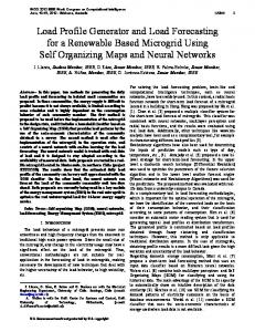
methods proposed in the literature to address this problem consist of heuristic techniques, statistical methods, and artificial intelligence-based techniques. Examples of the latter include fuzzy logic approaches, neural networks [5], or expert systems [6]. As for the statistical methods, they are usually classified as nonparametric [8], semiparametric, and parametric approaches. The latter may be based on a variety of methodologies, including linear regression; exponential smoothing [9]; stochastic time series [9], [10]; structural models; and state space models [11]. RTE has developed for more than 15 years a short-term load forecasting method that makes use of seasonal autoregressive integrated moving average (SARIMA) models. The method consists of the following steps. The load time series is first corrected from the influence of the weather by using a regression model, where the exploratory variables are the temperature and the nebulosity recorded in few selected cities and towns in France. The nebulosity is a measure of the cloud cover in real time. It influences the electricity consumption since it plays an important role in electric lighting consumption. The resulting adjusted series encompasses a general growth trend and several major cycles (daily, weekly, seasonal, yearly, etc.). Regarding the daily load curves, they can be classified in different groups corresponding to weekends, working days, non-working days, public holidays, and some special days. Furthermore, the load time series exhibit lasting abrupt changes in the stochastic pattern, termed breaks, for example due to public holidays and the transition periods between holidays and normal days. To illustrate the occurrences of these breaks, let us consider the load demand from Friday, April 27, 2007 to Monday, June 1, 2007, which are displayed in Fig. 1(a). We notice in this figure that there are several breaks appearing during the following time periods: Tuesday, April 30 and May 1; Monday, May 7 and Tuesday, May 8; Thursday, 17 and Friday, May 18, 2007 (approximately from observation 145 to 241, 481 to 577, and 961 to 1057). Interestingly, May 1, 8, and 18 are public holidays in France. Because the breaks do not follow the general pattern of the time series, they detrimentally affect the classical statistic approaches. To improve the robustness of the parametric forecasting methods, we may resort to a robust statistical estimation or a diagnostic approach. Good diagnostic techniques achieve robustness via outlier detection and hard rejection, resulting in missing values in the load time series. By contrast, robust methods accommodate outliers by bounding their influence on the estimates, yielding no missing values, which may be an advantage in some applications. In the robust statistical literature, there are numerous robust estimation methods that have

0885-8950/$26.00 © 2010 IEEE

CHAKHCHOUKH et al.: ELECTRIC LOAD FORECASTING BASED ON STATISTICAL ROBUST METHODS

983

SARIMA modeling for each of the 48 half-hours of a day that improves the quality of the forecast. The performances of our three proposed methods, namely RME, MHDE, and DEXR-based methods, are compared to those of the following approaches on the French electric load time series: 1) the classical maximum-likelihood-based estimation method of SARIMA models [17] applied after treating the outliers via a three-sigma rejection rule, which is denoted by corrected maximum likelihood (CML) method; 2) the robust filtered -estimator proposed by Yohai and Zamar [14]; 3) the generalized M-estimator (GM-estimator), which has been applied to power system state estimation by Mili et al. [18]. It is shown that while our three methods perform well in terms of robustness and forecasting accuracy, the RME-based procedure applied to the multivariate SARIMA models outperforms all the others due to its simplicity and small execution times. The paper is organized as follows. Section II is devoted to the analysis of the characteristics of the electric load in France and explains the modeling approach. Section III describes the proposed estimation methods for time series while Section IV provides some simulation results. Finally, Section V concludes the paper. II. CHARACTERISTICS OF THE ELECTRIC LOAD IN FRANCE

Fig. 1. (a) Half-hourly daily French electricity consumption on April 27 to June 1, 2007. (b) One-week differentiated French load time series at 10:00, 2009.

been proposed in linear regression with independent identically distributed (i.i.d.) errors [12], [13]. By contrast, only a handful of methods have been initiated in the correlated case of time series, which include the filtered -, filtered M-, generalized M-, and the so-called residual autocovariance (RA)-estimators of Bustos and Yohai [14], [15]. In this paper, we propose a diagnostic procedure for outlier and break detection and handling that makes use of two novel estimators for SARIMA parameter estimation and forecasting. The two estimators are termed the ratio-of-medians-based estimator (RME) and the minimum-Hellinger-distance-based estimator (MHDE). As an alternative to the SARIMA model, we investigate the double seasonal exponential smoothing with error correction [9], which is denoted by DEXN. This method being non-robust, we develop a new robust version, denoted by DEXR, which is inspired from the robust filter cleaner [14] and the robust exponential smoothing [16]. Furthermore, to deal with heteroscedasticity, we propose a simple novel multivariate

The method of forecast implemented at RTE accounts for the cyclic characteristics of the electric consumption. Three temporal cycles can be identified, namely 1) an annual cycle characterized by an annual peak demand in January and a dip on August 15; 2) a weekly cycle consisting of five working days with an overall stable consumption and the weekend, which is characterized by a decrease in the consumption; 3) a daily cycle; and 4) a general growth trend. Several parameters influence the electric consumption, which include meteorological factors, economical activities, and financial incentives for peak shaving via maximum load reduction tariffs, daylight saving time, and exceptional events. Because of all theses factors, the electrical consumption may be represented by a regular series containing the bulk of the observations and some outliers or “breaks”. A. Examples of Breaks in the Load Time Series To fix the ideas, let us give some examples of breaks in the differentiated load time series. Fig. 1(b) displays the one-week differentiated load time series at 10:00 in 2009, which is given for , where is the by consumption of the day at 10:00. We notice the presence of spikes at some sampling times, which are pinpointed by circles in the figure. Called outliers in statistics, these spikes stem from the abrupt changes in the differentiated load series from one day to the other over one week. Some of the circled points (days) are special days such as January 1, April 13, May 1 and 8, July 14, and December 25. Note that few special days cannot be noticed because of their appearance as weekends. August 15, November 1, and 11 are such days. Obviously, due to the qualitative change observed in the series during the breaks, it is of paramount importance to treat them separately from the majority of the data. In general, it is very difficult and challenging to detect these outliers by experience or visual inspection. This is because an

984


observation that is flagged as outlying relative to some model may not be deemed to be outlying relative to another model. Although the samples associated with the public holidays can be easily detected and deleted from the series, it is very difficult to state with precision the starting and the finishing points of the public holiday’s effect on the series. This explains why visual inspection can be either very robust but with a poor efficiency or efficient without being robust. For example, if the data analyst is too cautious and deletes longer segments than necessary of the series around a nonworking day, he may disregard good non-contaminated data points and thereby may induce a significant loss of efficiency of the estimation method by reducing the amount of data used. On the other hand, if the data analyst deletes too short segments around a break, he may retain outliers and thereby may induce a loss of robustness of the estimation method. Both cases will degrade the forecasting quality. Thus, there is a challenging tradeoff to achieve between high efficiency at the model of the majority of the samples (the Gaussian SARIMA model, in this case) and good robustness. This conflict can be better dealt with by relying on robust statistical theories and methods.

the number of periods is equal to 7 to model the within-week and are polynomials of order seasonal cycle; is a Gaussian white noise from . is the consumption of day at hour while corresponds to the half-hours . The residuals obtained from the SARIMA model at various hours are standardized via a robust estimator of scale. They are referred to as the standardized residuals. The standardized residuals of adjacent hours are correlated and their correlation is modeled by an ARMA model defined as

B. Modeling Time Series by SARIMA Forecasting load time series using SARIMA models is extensively used in the literature [3], [9]. In RTE, the day-ahead national load forecasting relies on a SARIMA applied to a dataset that has been corrected from climatic and financial incentives influence. The final predictions contain the forecast from the SARIMA added to the consumption based on climatic predictions and financial effects corrections. Because the SARIMA model has to be estimated online, quickness of execution of this task is critical. A double seasonal ARIMA model, SARIMA follows the equation

III. ROBUST ESTIMATING METHODS FOR TIME SERIES

where is the electricity demand at time and are is the number of periods in the different seasonal cycles; the lag operator; is the difference operator; and are the seasonal difference operators and are polynomials of order ; is a Gaussian white noise from . On the univariate half-hourly seequals 48 to model the within-day seasonal cycle, and ries to model the within-week cycle. In this paper, we propose an alternative modeling to deal with heteroscedasticity. Cast in a multivariate modeling framework, the electric consumptions are grouped according to half-hour time slots of the and represented by a vector day time series model that accounts for the correlation between adjacent series. We obtain 48 univariate series modeled by seasonal which folARIMA models, SARIMA lows the equation

(1) This model is used to improve the prediction. The series of the , where is residuals is given by the number of days in the series and is the residual of the day for the series of hour . The idea is to use the correlation between adjacent hours in the prediction without employing a too complex vector time series approach, which is difficult to develop and implement.

In this section, we introduce two novel robust methods to estimate contaminated Gaussian SARIMA models. A new robust multiplicative double seasonal exponential smoothing procedure is also proposed. A. Ratio-of-Medians-Based Estimator (RME) Our idea is to robustly estimate the autocorrelation and partial-autocorrelation functions, then to fit a high order AR model and filtering with this high order AR model to “clean” the data from the outliers, and finally to estimate an ARMA model in the presence of missing values. First, we show how to estimate the correlation in a Gaussian vector using sample medians, which are known for their robustwith covariness. Consider a zero mean Gaussian vector and ance matrix given by . The density of the product is given theoretically by

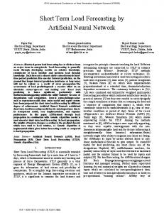
where is the modified Bessel function of the second kind [19]. The random variable follows a standard distribe the cumulative probability disbution of degree 1. Let and be that of . The ratio of tribution function of medians is expressed as

(2) is the median of . An explicit relation where between and does not seem to exist. Fig. 2 depicts as a , a relationship that is obtained numerifunction of cally.


985

we define the minimum-Hellinger-based estimator in the case of an AR(1) as

Fig. 2. Correlation coefficient of by (2).

X and Y versus the ratio of medians, , given

Consider now a Gaussian stationary time series and autocorrelation function . For each variance as we define

In order to improve the breakdown point of the estimator and prevent the appearance and the propagation of large outliers in the explanatory variables, which yield bad leverage points, we replace the prediction residuals by the robust prediction residuals. For an AR(1), robust prediction residuals are defined by and is obtained using a robust filter cleaner [24]. The proposed estimator is computed by the following steps: that minimizes the Hellinger cost Step 1) Search for function for a certain

with ,

(3) is the monovariate cumulative probability diswhere and is that of . The tribution function of sample median is defined as the median of the sample disof tribution function corresponding to a sample observations on . The sample medians and are calculated using the single ergodic and stationary time series . Then a robust estimate of is obtained by the relation . This estimator is called ratio-of-medians-based estimator (RME). To improve the efficiency of the model are estimated RME, the parameters of an ARMA via the following steps: using the RME, where is Step 1) Fit a high order AR selected by a robust order selection criterion subject to being larger than the order of the autoregressive part . Step 2) Detect the outliers by filtering with the high order , reject them, and use a classical maximum AR likelihood-based estimation method of ARMA models with missing values [20]. B. Minimum-Hellinger-Distance-Based Estimator (MHDE) The MHDE minimizes the Hellinger distance between a target density function and the empirical density function obtained from the observations [22]. This estimator offers the advantage of being as efficient as the maximum likelihood under the target probability distribution and very robust when the data observed deviates from the strict modeling assumptions [23]. using the Hellinger First, we show how to estimate and distance in the case of an AR(1) process given by , where . Minimizing the Hellinger distance of the prediction residuals with respect to both and gives multiple solutions and cannot be used for estimating the parameters. However, can be estimated by minimizing a robust efficient MHDE estimator of scale of the prediction residuals. Thus,

where is the nonparametric kernel estimate of the probability density function of the robust prediction residuals defined by

where is the number of observations used, is referred to as the kernel, and is a positive number known as the bandwidth [25]. The optimal choice of the bandwidth value and the kernel type are widely studied in the nonparametric area [25]. In this article, we propose to use a Gaussian kernel. that minimizes the Step 2) Choose the estimated previously. The algorithm proposed in this paper uses a simple grid search for , which is tractable since the interval of search is . To solve the MHDE estimator in a more general setting, more sophisticated optimization algorithms are described in [26]. , the MHDE-based estimator To estimate an AR with can be combined with a Durbin-Levinson algorithm to yield a robust-efficient Durbin-Levinson algorithm. This algorithm is given by • • • . are the robust residuals of the th step and obtained by the robust filter cleaner [24], [27]. The MHDE algorithm applied previously to estimate the in the case of an AR(1) will be used to estimate the partial autocorrelation funcat each step of the Durbin-Levinson algorithm. This tion in , calculate and means that for a certain that minimizes . This approach allows us choose the to estimate an autoregressive model of order , AR . model, we proTo estimate the parameters of an ARMA pose to use the same procedure as in Section III-A where in

986

step 1, the high order AR estimator.


is fitted using the MHDE-based

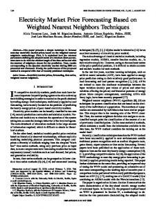
C. Robustness of the Proposed Methods The RME inherits its high robustness from that of the sample median, which is very resistant to outliers [12], [13]. As for the local robustness of the RME to infinitesimal contamination, it has been analyzed in [27] using a computed influence functional [14], [28]. The robustness and efficiency of the MHDE estimator has been studied in the paper of Lindsay [23]. Since the estimated scale of the residuals is robust and efficient, we conclude that the proposed filtered-MHDE-based estimator defined previously is robust. This estimator has the same approach as a filtered S-estimator as defined by [14]. To investigate further the robustness of the RME and the MHDE, we propose to compute next their maximum bias curves and derive their breakdown points. 1) Maximum Bias Curve and Breakdown Point of the Proposed Estimators: The maximum bias curves of the RME are calculated following the Monte Carlo procedure described in [14, p. 305]. For an AR(1), Fig. 3 depicts the maximum bias curve of our RME together with that of the GM estimator and the filtered MHDE. It is observed from these plots that the RME is robust and has a breakdown point (BP) of about 25%, that is, it can handle up to 25% of outliers among the data samples. The BP of an estimator of a parameter defined over a set is the maximum fraction of outliers contained in the data sample that this estimator can handle before reaching the bounds of the parameter set, which can be finite or infinite [14]. This BP is half of what the sample median can achieve in the location case beaffects two product cause for estimating , a single outlier and . The RME shows better performance terms, than the GM for . Furthermore, the BP of the GM decreases with increasing number of parameters to be estimated, a well-known result in robust statistics literature (i.e., [14]). On the other hand, our RME, being a continuous function of vari, exhibits a constant breakdown point regardables less of the order of the AR model. On the other hand, the filtered-MHDE has a maximum bias curve close to that of the RME-estimator. It has also a breakdown point larger to 25%, which seems to be constant regardless of the order of the AR model. This result is of great value since the percentage of outliers in load time series is around 10% to 15%. The efficiency of the proposed estimator can be verified empirically for an AR(1). We do this by calculating the variance of our estimator for increasing sample size . The efficiency is calculated using Monte Carlo replications of the sample. Table I shows that for , the efficiency of the filtered-MHDE-based estimator tends asymptotically toward unity with increasing . In order to assess the performance of the developed methods, we propose to compare them with two interesting robust estimators, namely, the Generalized M-estimator and the filtered -estimator. The GM estimator used in this article is given in [14], [29], and [30], where we propose to use the robust predicted residuals obtained with the robust filter cleaner. The filtered -estimates proposed by Yohai and Zamar [14], [31] are

Fig. 3. Maximum bias curves of three robust estimators of an AR(1) at

0:5.

=

TABLE I EFFICIENCY OF THE FILTERED-MHDE-BASED ESTIMATOR WITH INCREASING : SAMPLE SIZE n UNDER STANDARD GAUSSIAN DISTRIBUTION,

()

=05

obtained by minimizing the scale -estimates of the robust prediction residuals. The robust filtering is based on the state rep. The filter used is defined in [14] and resentation of an AR based on the robust filter of Masreliez [24], which is termed the filter cleaner. This filter adapts the outliers with their expected values from the other observations and the structure of the model. While at this stage, we can apply a maximum-likelihood estimator on the “cleaned” series, we prefer to delete the outliers and apply a classical estimator with missing values [20]. D. Robust Double Seasonal Exponential Smoothing The Holt Winters method is widely used in practice. It has the advantage of being simple. Taylor [9] gives a multiplicative formulation for the double seasonal Holt-Winters method, which is termed DEXN here. In the statistical literature, it is shown that the Holt-Winters method is not robust and some works suggest ways to robustify it [32], [16]. In this paper, we propose to robustify the approach used by [9] in the same spirit as the robust filter cleaner [14] and the robust exponential smoothing [16]. The obtained procedure, which is termed DEXR, is given by

where

is given by

(4)


Fig. 4. Day-by-day electricity demand in France for different hours from Saturday, January 1, 2005 to Sunday, January 2, 2006.

is the Huber -function and is a robust estimate of the scale of the one-step ahead forecast errors, which is assumed and to be constant. We estimate the parameters by minimizing the robust version of the mean squared forecast error (MSFE ), based for example on the -estimator of scale

(5) is a robust scale of the residuals such as an M-estimator or for example . IV. SIMULATION RESULTS In this section, we investigate via simulations the robustness and the forecasting quality of our proposed methods, namely the RME, the filtered-MHDE or F-Hel for short, and the DEXR, on the French electricity consumption time series. We compare their performances to those of three robust estimators proposed in the literature. The simulations are carried out as follows. The load demands under study are first corrected from the weather and the financial incentives effects. Then, a selection is made of the series over 100 weeks of half-hourly slots covering the period from Sunday, February 1, 2004 to Sunday, December 31, 2005. Fig. 4 displays the different electric consumption series for different half-hours. Observe the nonstationarity of the series and the presence of outliers, which makes the prediction of the electricity demand a very challenging task. Now, the first 70 weeks (February 1, 2004 to July 4, 2005) are used to estimate the parameters of the SARIMA model while the remaining 30 weeks are employed to evaluate the quality of the forecast up to 24 h ahead. This yields 490 observations for estimation and 210 observations for assessing the forecasts from 48 time series. The evaluation of the forecasting performance

987

is done via the mean absolute percentage error (MAPE). The MAPE values are computed up to ten days leading times. The series of the residuals contains 23 520 residuals for estimation and 10 080 for forecasting accuracy assessment. The forecasting evaluation is done over “normal” days, which makes the calculated MAPE values not sensitive to outliers or breaks. The proposed RME and MHDE methods are compared with the filtered- or F- for short, the GM-estimator, and the SARIMA estimation method applied after using the three sigma outlier rejection rule (CML). As previously explained, this rule consists in rejecting the samples that stand beyond three times a robust estimator of scale from a robust estimate of the trend (that is, the central part) of the time series. Furthermore, the proposed multivariate modeling approach is compared with the univariate approach based on the CML. The resulting MAPE values are displayed in Figs. 5 and 6. Fig. 5 depicts the MAPE for hours 8:00, 17:00, and 22:00. We notice that the improvement of the forecast varies from hour to hour. This is expected since some hours are more contaminated than others by outliers. For example, the time series in the night hours is not contaminated by non-working days. We can rank the methods from the best to the worst as follows: RME, F- , F-MHDE-based estimator, GM-estimates, and CML. The CML performs well for hours when there are no-outliers (22:00, for example). This is natural since the CML is based on maximum likelihood. The high efficiency of the RME, F- , and F-MHDE-based estimator is confirmed in the 22:00 series since they have a good performance, unlike the GM-estimator which lacks efficiency. For the 08:00 series, which possess several outliers, the differences in performance between the different robust and non-robust methods are apparent. Concerning the selected order of the high order autoregresof the 48 half-hourly weekly differentiated sive models AR series, we obtain the following results. For the RME estimator: is equal to 1 for 12 12 times the order 1 which means that time series, 2 times the order 2, once the order 3, once the order 6, 11 times the order 8, 13 times the order 9, 8 times the order 10. For the GM estimator: 3 times the order 1, 2 times 2, 14 times 7, 23 times 8, 3 times 9, 3 times 10. For CML estimator; once the order 8, 17 times the order 9, 4 times order 10, once the order 11 and finally 25 times the order 13. The orders differ from one method to the other and from half hour to another. This illustrates that the order selection is sensitive to the detection quality of outliers. The RME gives generally smaller orders of autoregressive (AR) models than the GM and the CML. For the RME, are small, which means we remark also that some values of that the autoregressive model is already fitting well our series and there is no need to fit an ARMA. Finally, the improvement in forecasting is due to better estimation of both the parameters and the orders of our models. In the case of the previously illustrated hours in Fig. 5, the obtained orders with the GM, RME, and CML are, respectively: 7, 10, 13 at 08:00. 7, 6, 13 at 17:00. 8, 10, 9 at 22:00. We remark that for 08:00, the order obtained with the RME is larger than the one obtained with the GM; still, the RME forecasts better than the GM the consumption at this hour. Fig. 6 displays the MAPE values of all the foregoing methods along with those of the univariate CML applied to a SARIMA

988


Fig. 6. Plot of MAPE versus the 48 half-hours (00 : 00; . . . ; 23 : 30) of a day for France (200 days post-sample period).

TABLE II ROBUST MEAN SQUARED ERROR OF THE FORECASTING ERROR AT LAG 1, RI ( 10 MW )

2 f

Fig. 5. Plot of MAPE forecast accuracy versus lead time: (a) 08:00, (b) 17:00, (c) 22:00 (200 days post-sample accuracy).

model with two seasonalities and . In this case, the traditional test of “outlyingness” of an observation is given by

(6) is the sample median of the double-differentiated series. . This test is based on the fact that . under standard normality, the probability . The traditional rule is discarding observations with Its MAPE is denoted by U3MADN in Fig. 6. From this figure,

g

it is clear that the proposed modeling and the robust methods improve the quality of forecasting. Fig. 7 displays the MAPE obtained with the proposed multivariate approach, which is denoted by MAPEC. Also are shown the MAPE values obtained without using the correlation between adjacent hours [i.e., using the ARMA model given by for all leading times. (1)]. We notice that Thus, as expected, considering the correlation between adjacent hours improves the forecasting of the series. Another interesting criterion to compare the forecasting quality of the foregoing methods is the error between the and its forecasted value from time observation at time (i.e., ). To this end, we compute the 200 out-of sample one-step-ahead forecast errors of the methods under , the MADN study. Then, we estimate the median , and calculate their robust mean squared error which is a robust index denoted by . The results are displayed in Table II. We observe that the RME, the filtered- , and the F-MHDE have similar performance. They are followed by the GM and finally the CML, which ranks last. Now, let us compare the forecasting quality obtained with the RME-estimated SARIMA when applied to the multivariate model with both the DEXN and DEXR. Table III shows the parameter estimates obtained via the two multiplicative exponential smoothing approaches. Fig. 8 displays the MAPE obtained


989

TABLE III PARAMETERS OF THE DOUBLE SEASONAL HOLT-WINTERS METHODS


Fig. 9. Half-hourly daily French electricity consumption and predictions on May 18, 2005.


when using the U3MADN based on the univariate SARIMA model, the RME and the CML, both based on the half-hour SARIMA multivariate model, and the DEXN and DEXR based on the univariate SARIMA model. It is apparent from this figure that the multivariate SARIMA-based methods perform better than both DEXN and DEXR. Note that the latter outperforms the classical DEXN, which is expected since the time series contains outliers. Note also that DEXN outperforms the three-sigma rejection univariate SARIMA model, U3MADN, which indicates that the latter is not very robust because it does not account for the correlation among the samples. It shows also that the classical exponential smoothing offers some robustness, especially towards spikes. Another important point worth mentioning is that the multivariate SARIMA model with one seasonality and one or two parameters to be estimated at each of the 48 half-hours of a day, which is obtained in this case, is quite simple and fast to identify using the proposed robust methods. Furthermore, the extra computing time that this model involves is worth spending in view of the improvement in the forecasting quality, which is significant. The relative computing times of the multivariate RME, multivariate GM-estimator, multivariate filtered- , univariate DEXR,

and multivariate filtered-MHDE are, respectively, 1, 1.5, 2, 5, and 50 for a series of load demands recorded every half-hour over 500 days. The processor used has a 1.6-GHz clock speed. Note that the developed programs are not optimized and are written using high level programming languages such as R or Matlab. These computing times can be substantially reduced if the algorithms are implemented in low-level programming languages or parallelized, for example on a half-hourly basis. The relatively high computing time of the filtered-MHDE is due to the fact that, at each step, we use a grid search by evaluating the . While cost function over 100 points within the interval the complexity of the algorithm is greatly reduced by combining the MHDE with the Durbin-Levinson procedure, it is still heavy to compute. Faster iterative algorithms are under development [26]. Regarding the univariate DEXR, we notice that it is five times slower than the multivariate RME. To give some insight about the improvements in the forecast provided by the developed methods, let us now investigate the forecast quality on the French daily consumption for one normal day. For example, we compare three of the main proposed methods, namely the multivariate RME, the univariate DEXR, and the U3MADN. Fig. 9 depicts the forecast of a normal day, Wednesday, May 18, 2005, following a break, Monday, May 16, 2005, which is a non-working day in France. It is apparent from that figure that it is difficult to assess the performance of these three methods via a simple visual inspection of the forecasts. However, this assessment can be easily carried out via a performance index evaluated over this day and defined as the sum of the 48 absolute errors of the forecast. This index is found to be equal to 9400 MW, 11 000 MW, 18 000 MW for the multivariate RME, the

990


DEXR, and the U3MADN, respectively. Obviously, the multivariate RME behaves better than the other two methods, especially the U3MADN. We evaluated also the forecast provided by these three methods of a normal day, Thursday, June 9, 2005, adjacent only to normal days. In that case, the sum of the 48 absolute errors of the forecast are equal to 8800 MW, 10 420 MW, and 10 400 MW for the multivariate RME, the DEXR, and the U3MADN, respectively. It is observed that, even if adjacent normal days are used in the forecast, the multivariate RME remains the best. This is because the estimation of the model that it provides, done over long segments of contaminated data, is less influenced by outliers. Finally, we conclude that the improvement is not only achieved on normal days following breaks but also on normal days following normal days. Note that the improvement of the forecast by robust methods is mild when it is carried out over one day. However, it becomes significant when it is carried out over a long period of days. Here, the assessment of the forecast quality has to be performed statistically. All the “normal days” forecasts are improved when the model is estimated robustly from the contaminated data. V. SUMMARY AND CONCLUDING COMMENTS The paper introduced three novel robust methods for shortterm load forecasting, namely the multivariate RME, the multivariate MHDE, and the univariate DEXR. Based on the concept of breakdown point, maximum bias curve, and simulation results, it has been shown that these methods are highly robust to outliers as well as to breaks present in the time series under study. Furthermore, they compare favorably with the filtered -estimators, the CML, and the GM estimators, which are robust methods proposed in the statistical literature. A performance assessment of all these methods has been carried out on real datasets consisting of French electricity demands over selected time periods. The conclusions that may be drawn from this investigation are the following. • The classical univariate estimation methods followed by the three-sigma hard rejection rule, which are widely used by practitioners, are not very robust when compared with the other robust methods studied in this work. Their weakness stems from the fact that these techniques do not account for the dependencies that exist among the samples of the series and, therefore, are unable to effectively detect some outliers and breaks. Consequently, these methods are not recommended. • The GM estimators [14], [18] are not as good as their competitors in terms of robustness and forecasting accuracy. Therefore, they are not advocated for this application. • The newly proposed univariate DEXR provides a more accurate and robust forecast of the French electricity demands than the classical DEXN. The DEXN has been recommended for load forecasting by Taylor [9]. This outcome is expected since the latter method is not robust to outliers and breaks while the former is. However, the DEXR is less accurate than the multivariate RME and, therefore, is not the preferred method.

• The multivariate filtered -estimator, which has been recently developed by Maronna et al. [14], presents very good performances on the French load forecasting. However, it is not straightforward to implement and is more time consuming than the multivariate RME. • The newly proposed multivariate MHDE is a very robust and highly efficient method. It has very attractive theoretical and practical features. However, it requires more computing time than the RME and, therefore, is recommended for offline application only. • The proposed RME-based multivariate approach using SARIMA models exhibits the best performances. It is this method that we recommend to use for online modeling and forecasting of the French load series. • In general, regardless of the estimation method being used, the proposed new multivariate modeling approach, which is simple and practical, has shown its effectiveness when applied to the French load forecasting. For example, the multivariate CML has better forecasting performance than its univariate counterpart (i.e., U3MADN). This is due to the fact this approach takes into account the heteroscedasticity of the series. Ongoing research effort has focused on the derivation of confidence intervals for the autocorrelations and, possibly, for the model parameter estimates obtained via the RME. A second research line is to seek a better and faster algorithm for the calculation of the MHDE-based estimates that is compatible with online applications. For instance, hybrid algorithms that combine gradient descent procedures with Newton’s method are of interest [26].

REFERENCES [1] G. Gross and F. D. Galiana, “Short-term load forecasting,” Proc. IEEE, vol. 75, no. 12, pp. 1558–1573, Dec. 1987. [2] H. K. Alfares and M. Nazeeruddin, “Electric load forecasting: Literature survey and classification of methods,” Int. J. Syst. Sci., vol. 33, pp. 23–34, 2002. [3] R. Weron, Modeling and Forecasting Electricity Loads and Prices: A Statistical Approach. New York: Wiley, 2006. [4] H. Hahn, S. Meyer-Nieberg, and S. Pickl, “Electric load forecasting methods: Tools for decision making,” Eur. J. Oper. Res., vol. 199, pp. 902–907, 2009. [5] H. S. Hippert, C. E. Pedreira, and R. C. Souza, “Neural networks for short-term load forecasting: A review and evaluation,” IEEE Trans. Power Syst., vol. 16, no. 1, pp. 44–55, Feb. 2001. [6] S. Rahman and R. Bhatnagar, “An expert system based algorithm for short term load forecast,” IEEE Trans. Power Syst., vol. 3, no. 2, pp. 392–399, May 1988. [7] N. Amjady and F. Keynia, “Short-term load forecasting of power systems by combination of wavelet transform and neuro-evolutionary algorithm,” Energy, vol. 34, pp. 46–57, 2009. [8] W. Charytoniuk, M. S. Chen, and P. Van Olinda, “Nonparametric regression based short-term load forecasting,” IEEE Trans. Power Syst., vol. 13, no. 3, pp. 725–730, Aug. 1998. [9] J. W. Taylor and P. E. McSharry, “Short-term load forecasting methods: An evaluation based on European data,” IEEE Trans. Power Syst., vol. 22, no. 4, pp. 2213–2219, Nov. 2007. [10] S. J. Huang and K. R. Shih, “Short-term load forecasting via ARMA model identification including non-Gaussian process considerations,” IEEE Trans. Power Syst., vol. 18, no. 2, pp. 673–679, May 2003. [11] V. Dordonnat, S. J. Koopman, M. Ooms, A. Dessertaine, and J. Collet, “An hourly periodic state space model for modelling french national electricity load,” Int. J. Forecast., vol. 24, no. 3, pp. 432–448, 2008.


[12] P. J. Rousseeuw and A. M. Leroy, Robust Regression and Outlier Detection, Wiley Series in Probability and Mathematical Statistics: Applied Probability and Statistics. New York: Wiley, 1987. [13] F. R. Hampel, E. M. Ronchetti, P. J. Rousseeuw, and W. A. Stahel, Robust Statistics: The Approach Based on Influence Functions, Wiley Series in Probability and Mathematical Statistics: Probability and Mathematical Statistics. New York: Wiley, 1986. [14] R. A. Maronna, R. D. Martin, and V. J. Yohai, Robust Statistics: Theory and Methods, Wiley Series in Probability and Statistics. Chichester, U.K.: Wiley, 2006. [15] O. H. Bustos and V. J. Yohai, “Robust estimates for ARMA models,” J. Amer. Statist. Assoc., vol. 81, no. 393, pp. 155–168, 1986. [16] S. Gelper, R. Fried, and C. Croux, “Robust forecasting with exponential and holt-winters smoothing,” Int. J. Forecast., vol. 29, no. 3, pp. 285–300, 2010. [17] G. E. P. Box, G. M. Jenkins, and G. C. Reinsel, Time Series Analysis: Forecasting and Control, Wiley Series in Probability and Statistics, 4th ed. Hoboken, NJ: Wiley, 2008. [18] L. Mili, M. G. Cheniae, N. S. Vichare, and P. J. Rousseeuw, “Robust state estimation based on projection statistics,” IEEE Trans. Power Syst., vol. 11, no. 2, pp. 1118–1127, May 1996. [19] , M. Abramowitz and I. A. Stegun, Eds., Handbook of Mathematical Functions With Formulas, Graphs, and Mathematical Tables. New York: Dover, 1992, reprint of the 1972 edition. [20] R. H. Jones, “Maximum likelihood fitting of ARMA models to time series with missing observations,” Technometrics, vol. 22, no. 3, pp. 389–395, 1980. [21] Y. Chakhchoukh, “A new robust estimation method for short-term load forecasting,” in Proc. Eur. Signal Processing Conf. (EUSIPCO), Glasgow, U.K., Aug. 2009. [22] R. Beran, “Minimum Hellinger distance estimates for parametric models,” Ann. Statist., vol. 5, no. 3, pp. 445–463, 1977. [23] B. G. Lindsay, “Efficiency versus robustness: The case for minimum Hellinger distance and related methods,” Ann. Statist., vol. 22, no. 2, pp. 1081–1114, 1994. [24] C. J. Masreliez and R. D. Martin, “Robust Bayesian estimation for the linear model and robustifying the Kalman filter,” IEEE Trans. Autom. Control, vol. AC-22, no. 3, pp. 361–371, Jun. 1977. [25] D. W. Scott, Multivariate Density Estimation: Theory, Practice, and Visualization, Wiley Series in Probability and Statistics. New York: Wiley, 1992. [26] P. A. D’Ambriosio, “A differential geometry-based algorithm for solving the minimum Hellinger distance estimator,” M.S. thesis, VirginiaTech, Balcksburg, 2008. [27] Y. Chakhchoukh, “A new robust estimation method for ARMA models,” IEEE Trans. Signal Process., vol. 58, no. 7, pp. 3512–3522, Jul. 2010. [28] R. D. Martin and V. J. Yohai, “Influence functionals for time series,” Ann. Statist., vol. 14, no. 3, pp. 781–855, 1986, with discussion.

991

[29] L. Denby and R. D. Martin, “Robust estimation of the first order autoregressive parameter,” J. Amer. Statist. Assoc., vol. 74, no. 365, pp. 140–146, 1979. [30] R. D. Martin, “Robust estimation of autoregressive models,” in Directions in Time Series (Proc. Meeting, Iowa State Univ., Ames, IA, 1978), Hayward, CA, 1980, pp. 228–262, Inst. Math. Statist. [31] V. J. Yohai and R. H. Zamar, “High breakdown estimates of regression by means of the minimization of an efficient scale,” J. Amer. Statist. Assoc., vol. 83, pp. 406–413, 1988. [32] T. Cipra, “Robust exponential smoothing,” Int. J. Forecast., vol. 11, no. 1, pp. 57–69, 1992.

Yacine Chakhchoukh (M’10) received the engineering degree (with honors) from Ecole Polytechnique d’Alger, Algiers, Algeria, in 2004 and the M.S. degree (with honors) in control and signal processing and the Ph.D. degree (with honors) from the University of Paris-Sud XI, Paris, France, in 2005 and 2010, respectively. From June 2006 to September 2009, he was with Gestionnaire du Réseau de Transport d’Electricite (RTE, the French transmission system operator), working on statistical robust signal processing for load forecasting. Currently, he is a Post-Doctoral Research Fellow with the Signal Processing Group at the Institute of Telecommunications, Technische Universität Darmstadt, Darmstadt, Germany, where he works on statistical robust estimation applied to practical problems such as communications.

Patrick Panciatici (M’00) received the engineering degree from the French Ecole Supérieure d’Electricité, Paris, France, in 1984. He joined EDF R&D in 1985, managing in EUROSTAG Project and CSVC project. He joined RTE, Versailles cedex, France, in 2003 and participated in the creation of the department “Methods and Support”. He is the head of a team that develops real-time and operational planning tools for RTE and ensures operational support on the use of these tools. Mr. Panciatici is a member of CIGRE, SEE, and the R&D ENTSO-E Working Group. He also is RTE’s representative in PSERC and several European projects (PEGASE, OPTIMATE, TWENTIES, etc.).

Lamine Mili (SM’90) received the electrical engineering diploma from the Swiss Federal Institute of Technology, Lausanne, Switzerland, in 1976 and the Ph.D. degree from the University of Liege, Liege, Belgium, in 1987. He is presently a Professor of electrical engineering at Virginia Tech, Blacksburg. His research interests include state estimation, transient stability, voltage collapse, and power system control.