A Fast Hue-Preserving Histogram Equalization Method for ... - CiteSeerX

A Fast Hue-Preserving Histogram Equalization Method for Color Image Enhancement using a Bayesian Framework D. Menotti∗†‡ , L. Najman∗ , A. de A. Araújo† , J. Facon‡ ∗ Institut

Gaspard-Monge, Université de Marne-la-Vallée,

Laboratoire A2SI, Groupe ESIEE Paris, Cité Descartes, BP99, 93162 Noisy-le-Grand, Île-de-France, France E-mail: {d.menotti,l.najman}@esiee.fr † Universidade

Federal de Minas Gerais, Departamento de Ciência da Computação

Núcleo de Processamento Digital de Imagens, Pampulha, Belo Horizonte, Minas Gerais, Brazil E-mail: {menotti,arnaldo}@dcc.ufmg.br ‡ Pontifícia

Universidade Católica do Paraná, Departamento de Informática

Programa de Pós-Graduação em Informática Aplicada, Padro Velho, Curitiba, Paraná, Brazil E-mail: {menotti,facon}@ppgia.pucpr.br

Keywords: histogram equalization, color image enhancement, hue preserving, Naive Bayes rule.

The remainder of this paper is organized as follows. Basic definitions for color images are presented in Section 2. Previous works related to our method are described in Section 3, and in Section 4 our new method is introduced. Experiments are shown in Section 5, and, finally, conclusions are drawn in Section 6.

Abstract – In this paper, we introduce a new hue-preserving histogram equalization method based on the RGB color space for image enhancement. We use R-red, G-green, and B-blue 1D histograms to estimate the histogram to be equalized using a Naive Bayes rule. The histogram equalization is performed by shift hue-preserving transformations. Our method has linear time and space complexities, which complies with realtime applications requirements. A subjective assessment comparing our method and other three is performed. Experiments showed that our method is more robust than the others in the sense that neither unrealistic colors nor over-enhancement are produced.

2. BASIC D EFINITIONS In this section, we present basic definitions for color images and its probability functions, which will be used throughout this work. Let N denote the set of natural numbers. Let X be a subset of points (x, y) ∈ N2 , such that 0 ≤ x < m, and 0 ≤ y < n, where m and n denote the dimensions of X. Let ||Y || denote the cardinality of a set Y ⊆ N2 . Note that ||X|| = m × n. A mapping I, from X to Z3L , is called an (color) image (in the RGB color space). We denote by I RGB such color image. In real applications, L is typically 256. Indeed, we have three mappings from X to ZL , which are the red, green and blue images, i.e., I R , I G and I B . For a point (x, y) ∈ X, Ri = I R (x, y), Gi = I G (x, y) and Bi = I B (x, y), are called the red, green and blue levels of the point (x, y) in I, respectively. We can RGB also denote (Ri , Gi , Bi ) by IR . In the following, we i ,Gi ,Bi define 1D, 2D and 3D histograms and probability density and distribution functions for color images. For the 1D case, we first consider the R color channel. IR Let HR be the absolute frequency of level Ro in image I R , o R where 0 ≤ Ro ≤ L − 1. The mapping H I from the levels R of image I R to its absolute frequency levels, i.e., H I : R ZL → N, is called the histogram of image I R . Let P I be the probability density function of I R . We denote by R R IR PRI o the probability of level Ro , i.e., PRI o = HR /m × n, o R where 0 ≤ Ro ≤ L − 1. Let C I be the cumulative density function (CDF, or the probability distribution function) of IR I R . We denote by CR the cumulative density of level Ro , Ro oI R IR i.e., CR = P ro =0 ro , where 0 ≤ Ro ≤ L − 1. It is o immediate to extend the above definitions of I R image, R R R i.e., H I , P I and C I , to I G and I B images. For the 2D case, we first consider the R and G color

1. I NTRODUCTION Image enhancement (IE) techniques have been often applied to Image Processing and Computer Vision applications in order to increase the probability of success in the image analysis task [2]. IE techniques are particularly useful in applications where an image with more distinguished texture details and perceptually better colors are required [3]. A great number of methods can be found in literature for the purpose of IE [3]. Among them, a well-known technique is Histogram Equalization (HE) [2]. HE consists of generating a uniform histogram (i.e., uniform distribution) from an original one. In image processing, the idea of equalizing the histogram of an image is to use the entire range of discrete levels of the image, stretching and/or redistributing the original histogram, such that an enhancement of image contrast is achieved. In this paper, we introduce a new hue-preserving HE method based on the RGB color space for IE. In fact, the proposed method is an extended and improved version of a previous work [4]. However, instead of using 3D or 2D histograms for IE, as in [5] and [4], we combine 1D histograms and a Bayesian framework [1]. Moreover, our method is hue-preserving [6], i.e., neither unrealistic nor new colors are produced after the enhancement process. The new method has linear time complexity with respect to both the image size and the number of discrete levels in each color channels. Hence, its complexity complies with real-time application requirements.

978-961-248-029-5/07 © 2007 UM FERI

433

2007 IWSSIP & EC-SIPMCS, Slovenia

RG

R

I channels. Let HR be the absolute frequency of Ri i ,Gi RG and Gi colors, in image I RG . The mapping H I from the levels of image I RG to its absolute frequency levels, RG i.e., H I : Z2L → N, is called the histogram of image RG RG be the probability density function of I . Let P I RG I RG . We denote by PRI i ,Gi the probability of (Ri , Gi ), i.e., RG RG I RG PRI i ,Gi = HR /m × n. Let C I be the CDF of I RG . i ,Gi RG I the cumulative density of (Ri , Gi ), We denote by CR i ,Gi  Ri Gi I RG I RG i.e., CRi ,Gi = ri =0 gi =0 Pri ,gi . It is immediate to RG extend the above definitions of I RB image, i.e., H I , RG RG PI and C I , to I RB and I GB images. For the 3D case, we have a single histogram and I RGB probability functions to be defined. Let HR be the i ,Gi ,Bi absolute frequency of Ri , Gi and Bi colors in image I. I RGB = 0 if there is no (x, y) ∈ X such Note that HR i ,Gi ,Bi RGB that I RGB (x, y) = (Ri , Gi , Bi ). The mapping H I from the levels of image I to its absolute frequency RGB levels, i.e., H I : Z3L → N, is called the histogram RGB RGB of image I . Let P I be the probability density RGB function of I RGB . We denote by PRI i ,Gi ,Bi the probability RGB I RGB of (Ri , Gi , Bi ), i.e., PRI i ,Gi ,Bi = HR /m × n. Let i ,Gi ,Bi RGB I RGB I RGB C be the CDF of I . We denote by CR i ,Gi ,Bi I RGB the cumulative density of (Ri , Gi , Bi ), i.e., CR = i ,Gi ,Bi Ri Gi Bi I RGB ri =0 gi =0 bi =0 Pri ,gi ,bi . In the next section, we present previous works related to the proposed method.

R

between ClO and ClI . In other words, the output level l for the input level l can be computed as the transformation R R R function T I (l), i.e., l = T I (l) = |(L − 1) × ClI |, where |z| stands for the nearest integer to z. To generate the output enhanced image with this transformation, for any pixel (x, y) ∈ X, we obtain the output value OR (x, y) R as l = T I (l), where l = I R (x, y). This method can easily be extended for color IE, by applying separately the equalization process described above to each I R , I G and I B images. This extended method produces a well-known problem; it produces unrealistic colors, since it is not hue preserving [6]. In the following, we call this extended method as the classical 1D HE for color IE. 3.2 3D Histogram Equalization The method proposed by Trahanias and Venetsanopoulos [5] takes into account the correlation of the three channels, R, G, and B, simultaneously. And it can can be described as follows. Let I and O be the input and output color images. RGB RGB RGB Let H I , PI and C I be defined as in SecO RGB tion 2. Let H be the uniform histogram of the output image, where any entry (Ro , Go , Bo ) has the same amount of pixels, since a such output histogram is desired, O RGB i.e., HR = L13 (m × n), or the same density, i.e., o ,Go ,Bo RGB PROo ,Go ,Bo = 1/L3 . And so, any entry (Ro , Go , Bo ) in RGB can be directly computed using its values Ro , Go CO and Bo , i.e.,

3. P REVIOUS W ORKS

(Ro + 1)(Go + 1)(Bo + 1) . (1) L3 To produce the output enhanced image, for any input pixel (x, y) ∈ X, where (Ri , Gi , Bi ) = I RGB (x, y), the smallest (Ro , Go , Bo ) is found for which the inequality

In this section we present works directly related to our proposed method. We first briefly describe the classical HE method for gray-level IE, which is extended for color images. We then show the 3D HE method proposed by Trahanias and Venetsanopoulos in [5], which is followed by a description of a 2D HE method recently proposed by us in [4]. These descriptions will help us to introduce our method in Section 4.

RGB

O = CR o ,Go ,Bo

RGB

RGB

I O − CR ≥ 0, CR i ,Gi ,Bi o ,Go ,Bo

(2)

is true. However this step presents an ambiguity since there exist many solutions for (Ro , Go , Bo ) that satisfy Equation 2. This ambiguity is remedied as follows. The RGB computed value of C I at (Ri , Gi , Bi ) is initially comRGB RGB pared to the value of C O at (Ro , Go , Bo )). If C I RGB is greater (resp. less) than C O , then the indexes Ro , Go , and Bo are repeatedly increased (resp. decreased), one at a time, until Equation 2 is satisfied. The obtained (Ro , Go , Bo ) is the output entry to (Ri , Gi , Bi ), i.e., if (x, y) ∈ x and (Ri , Gi , Bi ) = I RGB (x, y), then ORGB (x, y) = (Ro , Go , Bo ).

3.1 Classical 1D Histogram Equalization In this section we describe the HE method for monochrome images (e.g., gray-level or red ones), followed by its extension to deal with I RGB images. The goal of R HE is to uniformly distribute H I over the entire range of levels or, equivalently, to generate a CDF which increases monotonically as a straight line, such that an image contrast enhancement be achieved. The HE method for monochrome images is described as follows. Let I and O be the input and the output images, or the original and the equalized images, respectively. Let R R R R H I , P I and C I be defined as in Section 2. Let H O be the desired uniform histogram of the output image, where any level l has the same amount of pixels, i.e., R R HlO = L1 (m × n), or the same density, i.e., PlO = 1/L. R R Thus, the CDF C O is defined in function of l as ClO = l R I = (l + 1)/L. i=0 Pi  The l output equalized level corresponding to the input level l is obtained as the one that minimizes the difference

3.3 2D Histogram Equalization In this section, we describe the 2D HE method for Color IE, which is published in [4]. In this method, instead to use the correlation among the three channel as [5], it is used the correlation of channels two at a time. The method is described as follows. Let I and O be the input and output images. Let the input 2D histograms and probability functions be defined

434

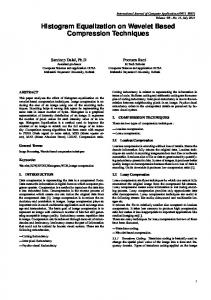
(a) Figure 1.

(b)

(c)

(d)

(e)

Results for the beach (partial Brazilian flag) image: (a) original image; (b) 1D HE; (c) 3D HE; (d) 2D HE; (e) our proposed method.

as in Section 2. Indeed, in this method, we do not equalize the three 2D histogram, but we equalize a 3D pseudoI RGB histogram, H  , which is defined based on a pseudo I RGB 3D CDF. This CDF, C  , is computed as the product of the three 2D CDFs for any entry (Ri , Gi , Bi ), i.e., I RGB

RG

RB

GB

I I I C  Ri ,Gi ,Bi = CR × CR × CG . i ,Gi i ,Bi i ,Bi

The method is based on the independence assumption of color channels, which is used in a Bayesian framework for computing the CDF. In Data Mining and Knowledge Discovery domains, it is well known that Bayesian classifiers work well, even though the independence assumption is violated [1]. Although it is also well known that this assumption does not hold for the R, G and B channels of color images, we hope that the enhancement produced in color image through HE will work well. We use 1D histograms to estimate a 3D probability distribution function, and then equalize the conceived histogram through the estimated function. The method is described as follows. Let I and O be the input and the output images, R G B R G B R respectively. Let H I , H I , H I , P I , P I , P I , C I , G B RGB C I and C I be defined as in Section 2. The CDF C I for any entry (Ri , Gi , Bi ) can be estimated as the product IB IG IB of every cumulative distribution CR , CG , and CB , i i i following the rule, i.e.,

(3)

The main rationale for computing this pseudo-CDF as the product of three 2D CDFs is that the three channels in an image are usually not simultaneously correlated. The output entry (Ro , Go , Bo ) for any pixel (x, y) ∈ X is computed as follows. Initially, (Ro , Go , Bo ) (the output triplet) is set up as (Ri , Gi , Bi ) = I RGB (x, y). Then an O RGB is computed by Equation 1, and an error initial CR o ,Go ,Bo is produced, i.e., I RGB

RGB

O C  Ri ,Gi ,Bi − CR . o ,Go ,Bo

(4)

This error will be used to guide the iterative process increasing or decreasing the output triplet (Ro , Go , Bo ). Note that as in [5], the solution for Equation 4 also presents an ambiguity. There are several solutions for (Ro , Go , Bo ) that satisfy Equation 1. Instead to increase or decrease each channel at a time by a unit, the channels are increasing or decreasing by proportional factors based on each channel (for details, see [4]). The rationale for this is that we can stretch the histogram simultaneously in all three direction by factors depending on their-self. The output triplet (Ro , Go , Bo ) is the nearest integer triplet which approximates to zero the difference between the I RGB O RGB CDFs C  and C  , i.e., Equation 4. Note that this HE method is not hue preserving, since the shift transformation performed from (Ri , Gi , Bi ) to (Ri + k × TR , Gi + k × TG , Bi + k × TB ) ≈ (Ro , Go , Bo ) is not hue preserving [6], where TR , TG and TB stands for the displacement taken for each channel and k is the number of iterations required to find the miminum error in Equation 4. The hue is not preserved because we may take different displacements in each directions. In the next section, we present our proposed method.

I RGB

R

G

B

I I I C  Ri ,Gi ,Bi = CR × CG × CB . i i i

(5)

I RGB

Note that in this equation, C  obeys a Naive Bayes I RGB sense, whilst in Equation 3 C  is defined without a mathematical mean. Unlike to iteratively increase or decrease Ro , Go and Bo , in order to minimize Equation 4 as performed in the method described in Section 3.3, we propose to find the output triplet (Ro , Go , Bo ) for any image pixel in a single step, i.e., O(1). From Equations 4 and 1 or for solving Equation 5, we have (Ro + 1)(Go + 1)(Bo + 1) = 0. (6) L3 If we take Ro , Go and Bo as Ri + k, Gi + k and Bi + k, respectively, where k is the number of iterations required for minimizing Equation 4, we obtain I RGB

C  Ri ,Gi ,Bi −







k 3 + k 2 [Ri + Gi + Bi ]+       k[Ri × Gi + Ri × Bi + Gi × Bi ]+ 





3

Ri × Gi × Bi − L × 





RGB

I C  Ri ,Gi ,Bi

(7)

= 0.

where Ri , Gi , and Bi means Ri + 1, Gi + 1, and Bi + 1, respectively. By solving this a cubic equation in function of k, we obtain the desired output triplet (Ro , Go , Bo ) as the input one plus the displacement k, i.e., (Ri + |k|, Gi + |k|, Bi + |k|), where |k| stands for the nearest integer to k. Equation 7 can easily be solved by Nickalls [7] or by classical Cardian methods using transcendental functions. It would be preferred to use the Nickalls method, since it is faster and mathematically simpler than the last one.

4. T HE PROPOSED METHOD In this section, we present a hue-preserving HE method based on the RGB color space for IE. Indeed, this method is an extended and improved version of the method proposed in Section 3.3. It is linear with respect to both the image size and the number of discrete levels in each channel.

435

(a) Figure 2.

(b)

(c)

(d)

(e)

Results for the train image: (a) original image; (b) 1D HE classic; (c) 3D HE; (d) 2D HE; (e) our proposed method.

6. C ONCLUSION

Note that any image pixel is equalized following a shift transformation by a k factor, i.e., (Ri , Gi , Bi ) to (Ri + |k|, Gi + |k|, Bi + |k|), which is hue preserving [6]. Hence the proposed method is also hue preserving.

In this paper, we introduced a new hue-preserving HE method based on the RGB color space for IE. The proposed method has O(max(m × n, L)) and O(L) time and space complexities, respectively. Such method complies with real-time application requirements, given its complexities. Although the classical 1D HE method is six times faster than ours, it is not hue preserving. Remark that our method is two and forty times faster than the 2D and 3D HE ones, respectively. In practice, our method enhances 1024×1024 image pixels in 100 milliseconds on a Pentium 4 - 2GHz. As shown on the experiments in the previous section, it is difficult to judge an enhanced image result even with a subjective assessment. However, we claim that our method is more robust than the others in the sense that neither unrealistic colors nor overenhanced are produced. For future works, we plan to evaluate the methods using naturalness and colorfulness metrics [8] on a database with hundreds of images collected from internet, such that a quantitative comparison can be performed.

5. E XPERIMENTS

In this section, a comparison among our proposed HE method and the 1D [2], the 3D [5], and the 2D [4] methods is carried out. A subjective assessment is carried out to compare the visual quality of the images. Here we discuss results for two images. Figure 1 shows the results for the first image, the beach. Note that unrealistic colors are present in the image generated by the 1D HE method (Figure 1(b)). The image produced by the 3D HE method is overenhanced, producing colors very saturated (Figure 1(d)), i.e., bright colors. In turn, the image produced by the 2D HE method (Figure 1(d)) is more realistic than the others. In contrast, another type of judgement can be performed considering the application. We can say that the resulted image of the 3D HE method has better quality than the others, since the water region in the image was better enhanced. Despite of these arguments, we can say that our method generates an image (Figure 1(e)) with a good balance between non saturated and realistic colors.

ACKNOWLEDGMENTS We would like to acknowledge support for this research from UFMG, PUCPR, CAPES/MEC, CNPq/MCT.

R EFERENCES [1] P. Domingos and M. Pazzani, “On the optimality of the simple bayesian classifier under zero-one loss,” Machine Learning, vol. 29, no. 2-3, pp. 103–130, 1997. [2] R. Gonzalez and R. Woods, Digital Image Processing, 2nd ed. Prentice Hall, Jan. 2002. [3] K.-Q. Huang and Q. Wang and Z.-Y. Wu, “Natural color image enhancement and evaluation algorithm based on human visual system,” Computer Vision and Image Understanding, vol. 103, pp. 52–63, 2006. [4] D. Menotti, A. P. Melo, A. de Albuquerque Araújo, J. Facon, and E. M. Sgarbi, “Color image enhancement throught 2D histogram equalization,” in 13th IWSSIP, Budapest, Hungry, 21-23 September 2006, pp. 235–238. [5] P. Trahanias and A. Venetsanopoulos, “Color image enhancement through 3-d histogram equalization,” in Proceedings of 11th International Conference on Pattern Recognition (ICPR). IEEE, 1992, pp. 545–548. [6] S. Naik and C. Murthy, “Hue-preserving color image enhancement without gamut problem,” IEEE Tran. on Image Processing, vol. 12, no. 12, pp. 1591–1598, Dec. 2003. [7] R. Nickalls, “A new approach to solving the cubic: Cardan’s solution revealed,” The Mathematical Gazette, vol. 77, pp. 354–359, 1993. [8] S. Yendrikhovskij, F. Blommaert, and H. de Ridder, “Perceptually optimal color reproduction,” in Proc. of SPIE: Human Vision and Elec. Imag. III, vol. 3299, 1998, pp. 274–281.

Figure 2 shows the results for the second image, the train. We observe that the 3D HE method produces an overenhanced image (Figure 2(c)), that is, the colors are very saturated. Our method and the 2D one produce images (Figure 2(d)) better enhanced than the one obtained by the 3D HE method. However, some hidden details in dark regions continue to be uncleared. In our opinion, the best enhancement is achieved by the image produced by the 1D HE method (Figure 2(b)). In this case, the image produced by the 1D HE method presents colors which are more realistic for the green regions and have more details than those produced by the other three methods. However, again, note that in the sky portion of the image, unrealistic colors are produced by the 1D HE method. From the discussion above, we claim that our method produces images (Figures 1(e) and 2(e)) with the best tradeoff between the enhanced colors and saturation. That is, our method produces images with colors that are more realistic than the 1D and 2D HE methods (which are not hue preserving), and the images are not so saturated as the ones produced by the 3D HE method.

436