Evaluation of Quantile Based Histogram Equalization with ... - CiteSeerX

Evaluation of Quantile Based Histogram Equalization with Filter Combination on the Aurora 3 and 4 Databases Florian Hilger and Hermann Ney Lehrstuhl f¨ur Informatik VI RWTH Aachen – University of Technology Ahornstr. 55 52056 Aachen, Germany

fhilger,

g

ney @informatik.rwth-aachen.de

Abstract The recognition performance of automatic speech recognition systems can be improved by reducing the mismatch between training and test data during feature extraction. The approach described in this paper is based on estimating the signal’s cumulative density functions on the filter bank using a small number of quantiles. A two–step transformation is then applied to reduce the difference between these quantiles and the ones estimated on the training data. The first step is a power function transformation applied to each individual filter channel, followed by a linear combination of neighboring filters. On the Aurora 4 16kHz database the average word error rates could be reduced from 60.8% to 37.6% (clean training) and from 38.0% to 31.5% (multi condition training).

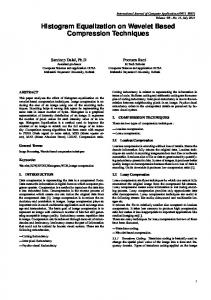
1. Introduction Quantile based histogram equalization [1] [2] is an approach to reduce the mismatch between the training and test conditions of an automatic speech recognition system during feature extraction. The cumulative density functions of the signals after the Mel–scaled filter bank are determined within a moving window and approximated by a few, typically NQ = 4, quantiles (Figure 1). This approach can be used for online applications [1] that only allow a short delay. 100

2. Power function transformation In the implementation investigated here the quantile equalization was applied to the output of the Mel–scaled filter bank [1]. The usual logarithmic compression of the dynamic range was replaced by a 10th root compression which in most cases lead to better baseline error rates on the noisy databases it was tested on [2]. The first transformation step is a power function with an additional linear term that is applied to each individual filter channel [1]. In the following equations Yk is the output of the k-th filter. Tk is the transformation function with the corresponding transformation factors  and . The recognition quantiles are denoted Qk;i were i is the quantile’s index. Note that in the online implementation all these variables depend on time, but additional index t is not used here to keep the notation more readable.

Tk (Yk ) = 

Qk;NQ k



Yk

 k

Qk;NQ

k )

+ (1

Yk



(1)

Qk;NQ The original values are scaled to the interval [0; 1℄, dividing by the largest quantile Qk;NQ . In the online implementation scaling up Qk;NQ with a factor e.g. 1.5 can improve the recognition performance. After the transformation the values are scaled back to their original range. The transformation  and parameters are chosen to minimize the squared distance between the current quantiles and the ones estimated on the training data Qtrain . i

75

%

The difference between the reference quantiles, estimated on the training data, and the current quantiles in recognition is then minimized with an appropriate transformation function. In the following a two step transformation will be described.

50

0

NX Q 1

f k ; k g = argmin 

25

f k ;k g

clean noisy 0 1

1.5

2

2.5

Y

Figure 1: Cumulative density functions of the 10th filter output with 25% quantiles for clean and noisy speech data (Aurora 4 test sets 1 and 8).

i =1

Tk (Qk;i ) Qtrain i

2

1 A (2)

A grid search is carried out to find the optimal values of  and . In the online implementation the values have to be updated every time frame. To reduce the search effort and avoid rapid changes of the parameters that can deteriorate the recognition performance by inducing insertion errors, the updated values are only searched within a small range 0:01 from the previous values [1].



3. Combination of neighboring filter channels

before quantile equalization 2.8

T~k (Q~ k;i ) = (1 k k )Q~ k;i + k Q~ k 1;i + k Q~ k+1;i

(3)

2.6 clean signal (test set 1)

The combination of neighboring filter channels as second normalization step was introduced in [2]. The idea is to linearly combine each filter with its left and right neighbor to take pos~ k;i are the recognition sible dependencies into account. Here Q quantiles after applying the preceding power function transformation.

fk ; k g

=

NX Q 1

argmin 

fk ;k g

i =1

T~k (Q~ k;i ) Qtrain i

2.2 2 1.8 1.6 1.4 1.2 1

The combination factors k and k are chosen to further reduce the squared distance between the training and the recognition quantiles. 0

2.4

0.8 0.8

1

1.2

1.4

1.6

1.8

2

2.2

2.4

2.6

2.8

signal with car noise (test set 8)

Figure 2: Output of the 10th Mel–scaled filter. Data with car noise and microphone mismatch (test set 8) before quantile equalization plotted against original clean data (set 1).

2

1

2 2
+ k + k A

after quantile equalization

(4)

2.8

The factor in Equation 4 is a penalty which ensures that the values k and k remain small, i.e. below 0.1. If they are not restricted the recognition performance will deteriorate. Figures 2 and 3 are examples that show the influence of quantile equalization with filter combination on the noisy data. The 166 utterances of the Aurora 4 noisy Wall Street Journal (WSJ) test data were used to generate the scatter plots of the output from the 10th filter (of 23). Each point corresponds to one time–frame of the test data. The data with car noise (test set 8) is plotted against the original clean data (set 1). If there was no mismatch between the two test sets, all points should lie on the diagonal. If a point lies below the diagonal the magnitude of the noisy signal is higher than the one of the corresponding clean signal. Figure 2 shows the situation before quantile equalization: the high magnitude speech portions of the signal scatter around the diagonal, while the low magnitude silence portions of the signal are clearly shifted below the diagonal. This shows that the mismatch in the silence portions of the signal is especially large. Figure 3 shows the data after quantile equalization with filter combination. The resulting “cloud” of points is narrower and silence region is shifted closer to the diagonal. Even though the speech parts of the signal now all lie above the diagonal, the average horizontal distance from the diagonal

d=

T  1 X

T t=1

Y10 ar [t℄ Y10 lean [t℄

2

(5)

is significantly reduced. In the equation Y10 [t℄ is the output of the 10th filter at time t for the lean and ar test sets, T is the total number of time–frames. While d = 101 10 3 for the points shown in Figure 2 it is reduced to 56 10 3 in Figure 3. If quantile equalization is used without filter combination, the scatter plot does not look significantly different and the corresponding average distance is only slightly higher (57 10 3 ), but even this small difference can still have an impact on the resulting recognition error rates. (Tables 5 and 6).










clean signal (test set 1)

2.6 2.4 2.2 2 1.8 1.6 1.4 1.2 1 0.8 0.8

1

1.2

1.4

1.6

1.8

2

2.2

2.4

2.6

2.8

signal with car noise (test set 8)

Figure 3: Output of the 10th Mel–scaled filter. Data with car noise and microphone mismatch (test set 8) after quantile equalization plotted against original clean data (set 1).

4. Recognition results Database definitions: Recognition tests were carried out on the Aurora 3 and 4 databases provided by ELRA. Aurora 3 consists of digit string subsets from the SpeechDat–Car databases in Danish, Finnish, German, and Spanish. The data was recorded in real car environment with a sampling rate of 8kHz. Different noises with an average SNR of 10dB were added to the Wall Street Journal 5k database to generate the Aurora 4 database [3]. Data with 8kHz and 16kHz sampling rate is available. It was not the intention of this work to evaluate voice activity detection algorithms so the endpointed test data was used, 200ms of silence were left before and after each utterance. Feature extraction: to make the conclusions drawn from the experiments comparable the same modified version of the Aurora WI007 MFCC feature extraction front end [4] was used for both databases.

  

Aurora WI007 MFCC feature extraction front end [4] Logarithm replaced by 10th root Quantile equalization and mean normalization module

 

added between 10th root and the calculation of the cepstral coefficients Quantile Equalization applied only during recognition Moving window online implementation with – 10ms delay and 5s window length for Aurora 3 – 1s delay and 5s window length for Aurora 4

  

0th cepstral coefficient used instead of log energy 13 cepstral coefficients with first and second derivatives No feature vector compression

Aurora 3 SpeechDat–Car recognizer setup: the baseline HTK recognizer setup described in [5] was used without modification:

    

HTK speech recognition toolkit (old Aurora evaluation settings [5]) Gender independent models Word models of fixed length (16 states) for the digits 552 Gaussian mixtures densities

    

baseline WM MM HM Avg

ISIP speech recognition system (Aurora evaluation settings [3]) Gender independent models 3215 context dependent triphone states tied using decision trees 12.9k Gaussian mixture densities Across word modeling Bigram language model

Aurora 4 noisy WSJ recognition results: recognition tests were conducted on the 8kHz and 16kHz sampling rate data. Both training sets were used. The results are shown in Table 5 and 6. Like in the previous tests the average word error rates was significantly reduced by simply applying 10th root compression and mean normalization.

Word Error Rates [%] Finnish Spanish German Danish Average 7.3 7.1 8.8 12.7 9.0 19.5 16.7 19.0 32.7 22.0 59.4 48.5 26.8 60.6 48.9 24.6 20.8 16.9 31.7 23.5

Table 2: 10th: 10th root compression and mean normalization. 10th WM MM HM Avg

No language model

Aurora 3 SpeechDat–Car recognition results: a detailed overview over the recognition results for different setups is shown in the Tables 1–4. The average baseline word error rate is 23.5% (Table 1). Simply applying 10th root compression and mean normalization reduced the average word error rate to 15.4% (Table 2). Applying quantile equalization further improves the result leading to an error rate of 13.7% (Table 3). The combination of neighboring filters did not meet the expectations. The improvements observed in previous tests on other databases [2] could not be reproduced here, the average error was 13.7% again. When comparing the recognizer setup for the Aurora 3 experiment with the setups for the other databases described in [2], the difference in the acoustic modeling stands out. For the Aurora 3 baseline test all digit models for all languages had the same number of states, only three mixture densities per state were used and the amount of training data was quite small. Apparently, the combination of neighboring filters only has a positive effect on the error rate if the acoustic models are better. The following tests on Aurora 4 will underline this assumption. Aurora 4 noisy WSJ recognizer setup: all tests on the noisy WSJ 5k database were carried out with the reference system [3] provided by Mississippi State University’s Institute for Signal Processing (ISIP):



Table 1: Baseline Recognition results for the Aurora 3 SpeechDat–Car databases. 8kHz sampling rate, endpointed data. WM: well matched, MM: medium mismatch, HM: high mismatch, Avg: weighted average (0.4WM+0.35MM+0.25HM).

Word Error Rates [%] Finnish Spanish German Danish Average 4.9 8.2 8.3 14.8 9.0 12.5 11.2 17.8 28.0 17.4 26.1 17.5 17.7 29.6 22.7 12.9 11.6 13.9 23.1 15.4 Table 3: QE: quantile equalization.

10th QE WM MM HM Avg

Word Error Rates [%] Finnish Spanish German Danish Average 4.5 7.8 7.5 12.4 8.1 12.1 10.1 16.5 23.5 15.5 20.1 16.5 16.5 26.6 19.9 11.1 10.8 12.9 19.8 13.7

Table 4: QEF: quantile equalization with filter combination. 10th QEF WM MM HM Avg

Word Error Rates [%] Finnish Spanish German Danish Average 4.5 8.0 7.6 12.1 8.0 12.2 10.1 16.8 23.4 15.6 20.6 16.4 16.6 26.8 20.1 11.3 10.8 13.1 19.7 13.7

Filter specific quantile equalization did consistently reduce the average word error rates on the 8kHz data (Table 5), but the effect was fairly small. In these experiments the combination of neighboring filters had larger effect on the error rates, even though the impact on the squared distance form the clean data (Equation 5) was much smaller. On the 16kHz data the situation is different. When training on clean data quantile equalization of independent filters reduced the average error rate by an absolute 1.7% the combination of filters only contributes an insignificant 0.1%. In the multi condition test each transformation step had a contribution of 0.6% absolute word error rate reduction. In total, the average word error rate could be reduced form 57.9% to 40.3% for 8k clean training, from 38.8% to 32.9% for 8k multi condition training, from 60.8% to 37.6% for 16k clean training, and from 38.0% to 31.5% for 16k multi condition training. So as to be expected, the largest relative error rate reductions were observed when the system was trained on clean data, the lowest absolute error rates when training on multi condition data. A closer look at individual noise conditions shows that the approach described in this paper yields the highest error rate reductions on the test sets with the stationary car noise (2 and 9).

Table 5: Recognition results for the Aurora 4 noisy WSJ databases without feature vector compression. 8kHz sampling rate, endpointed data. 10th: 10th root and mean normalization, QE: quantile equalization, QEF: quantile equalization with filter combination. train. data clean

multi cond.

8kHz setup baseline 10th 10th QE 10th QEF baseline 10th 10th QE 10th QEF

1 16.2 15.8 15.6 15.3 18.4 23.5 22.6 21.4

2 49.6 22.3 22.2 21.5 24.9 21.8 22.4 21.4

3 62.2 42.0 41.8 39.9 37.6 31.3 31.0 30.3

4 58.7 45.4 45.0 44.3 39.3 35.9 36.4 35.5

5 58.2 45.7 43.3 42.3 38.8 36.6 36.4 35.0

6 61.5 43.9 44.4 42.8 38.2 33.8 34.5 33.0

Word Error Rates [%] test set 7 8 9 61.7 37.4 59.7 47.7 26.2 34.0 46.0 25.4 33.4 45.2 24.3 31.0 40.4 29.7 37.3 37.8 25.9 29.2 36.2 24.5 28.3 37.0 22.9 27.6

10 69.8 51.7 51.1 48.4 48.3 39.2 39.3 38.2

11 67.7 54.2 53.9 51.6 46.1 41.9 42.5 40.2

12 72.2 56.5 56.1 54.9 50.6 42.1 42.2 40.8

13 68.3 51.8 51.6 49.0 44.9 37.3 37.8 36.0

14 67.9 54.9 53.9 53.2 49.3 41.9 41.8 40.8

Avg. 57.9 42.3 41.7 40.3 38.8 34.2 34.0 32.9

Table 6: Recognition results for the Aurora 4 noisy WSJ databases without feature vector compression. 16kHz sampling rate, endpointed data. 10th: 10th root and mean normalization, QE: quantile equalization, QEF: quantile equalization with filter combination. train. data clean

multi cond.

16kHz setup baseline 10th 10th QE 10th QEF baseline 10th 10th QE 10th QEF

1 14.0 14.5 14.0 13.4 19.2 21.4 20.5 19.9

2 56.6 18.9 19.1 18.7 22.4 18.3 18.1 17.7

3 57.2 33.4 31.6 31.8 28.5 24.2 24.3 24.1

4 54.3 41.1 38.0 37.6 34.0 30.0 28.9 29.0

5 60.0 37.5 34.5 36.1 34.0 26.2 25.3 25.0

6 55.7 34.8 33.0 31.8 30.0 25.4 25.6 25.6

Word Error Rates [%] test set 7 8 9 62.9 52.7 74.3 38.7 32.8 38.9 37.3 31.5 37.7 36.9 30.3 37.7 33.9 45.0 43.9 29.7 32.5 35.5 29.5 32.2 33.6 28.9 29.8 33.0

10 74.3 49.4 47.3 47.6 47.2 41.8 41.7 39.8

11 67.5 52.3 50.5 50.5 46.3 42.8 42.5 42.2

12 75.6 56.7 53.9 54.4 51.2 45.2 43.5 43.8

13 71.9 48.3 48.1 47.6 46.6 41.3 40.8 40.4

14 74.7 53.8 51.0 52.0 50.0 43.4 42.3 42.6

Avg. 60.8 39.4 37.7 37.6 38.0 32.7 32.1 31.5

5. Conclusions

6. Acknowledgements

This paper has presented detailed investigations on the influence of different normalization steps on the Aurora 3 and 4 databases. On both datasets considerable error rate reductions were obtained by simply applying 10th root compression and mean normalization. On the Aurora 3 SpeechDat–Car databases quantile equalization of individual filter channels could further reduce the average word error rate from 15.4% to 13.7%. A combination of neighboring filters did not have any additional effect, presumably because the acoustic modeling was not detailed enough to be significantly influenced by the small combination factors. Further experiments to underline this assumption will have to show if the effect of filter combination is really related to the number of densities that are trained. In terms of relative word error rate reduction the effect of quantile equalization was smaller on the Aurora 4 database. But filter specific quantile equalization and the combination of neighboring filters were both able to contribute to the improvement. Putting everything together the average word error rates were reduced from 60.8% to 37.6% (clean training) and from 38.0% to 31.5% (multi condition training) on the 16kHz subset. Tests with the RWTH large vocabulary speech recognition system are planned to show which error rates can be obtained when the restriction of a standardized recognizer is dropped, and the feature extraction front end is optimized together with the back end.

This work was partially funded by the DFG (Deutsche Forschungsgemeinschaft) under contract NE 572/4-1

7. References [1] F. Hilger, S. Molau, and H. Ney, “Quantile Based Histogram Equalization for Online Applications,” in Proc. of the 7th International Conference on Spoken Language Processing, Denver, CO, USA, Sept. 2002, vol. 1, pp. 237–240. [2] F. Hilger, S. Molau, and H. Ney, “Combining Neighboring Filter Channels to Improve Quantile Based Histogram Equalization,” in Proc. IEEE International Conference on Acoustics, Speech, and Signal Processing, Hong Kong, China, Apr. 2003, vol. I, pp. 640–643. [3] N. Parihar and J. Picone, “DSR Front End LVCSR Evaluation AU/384/02,” Tech. Rep., ETSI Aurora Working Group, Sophia Antipolis, France, Dec. 2002. [4] ETSI ES 201 108 V1.1.2, “Speech Processing, Transmission and Quality aspects (STQ); Distributed speech recognition; Front–end feature extraction algorithms; Compression algorithms,” Tech. Rep., ETSI, Sophia Antipolis, France, Apr. 2000. [5] H.-G. Hirsch and D. Pearce, “The Aurora Experimental Framework for the Performance Evaluation of Speech Recognition Systems Under Noisy Conditions,” in ASR2000 – International Workshop on Automatic Speech Recognition, Paris, France, Sept. 2000, pp. 181–188.