ABSTRACT. A novel color histogram equalization approach is proposed that not only takes into consideration the correlation between color components in the ...
COLOR HISTOGRAM EQUALIZATION USING PROBABILITY SMOOTHING Nikoletta Bassiou and Constantine Kotropoulos Department of Informatics, Aristotle University of Thessaloniki Box 451 Thessaloniki 541 24, GREECE phone: + (30) 2310996361, fax: + (30) 2310998453, email: {nbassiou, costas}@aiia.csd.auth.gr
ABSTRACT A novel color histogram equalization approach is proposed that not only takes into consideration the correlation between color components in the color space, but it is also enhanced by a multi-level smoothing technique adopted from the field of language modeling. In this way, the correlation between color components is taken into account and the problem of unseen values for a color component, either considered independently or in combination with others, is efficiently dealt with. The proposed method is conducted in the HSI color space for intensity (I) component and saturation (S) component given the I component. The quality of the visually appealing equalized images was confirmed by means of the entropy and the Kullback-Leibler divergence estimates between the resulted color histogram and the multivariate uniform probability density function. 1. INTRODUCTION Image enhancement has as main task to improve the visual quality of an image from the human perspective. It uses several techniques, such as histogram equalization, contrast stretching, and slicing, that were initially developed for grayscale images. However, several attempts have been made to generalize the aforementioned techniques to color images. The generalization has been proven to be rather complicated due to the various color models and the relationships between the color components. Histogram equalization being the most simple and effective method for enhancing the contrast of an image was one of the fields where a non-trivial, but not always successful generalization from gray-scale images to color images has been observed. As expected, the literature on color histogram equalization is not as rich as that on gray-scale histogram equalization. The most simple and straightforward extension is the application of gray-scale histogram equalization to the different bands of the color image. Some efforts were also focused in spreading the histogram along the principal component axes of the original image [1] or spreading repeatedly the three two-dimensional histograms [2]. In [3, 4], histogram equalization is mainly based on the brightness component of the original color image. Since the aforementioned techniques use only marginal color histograms, the correlation between the different color bands is ignored. Latter methods tried to exploit the correlation between color components. For example, the cumulative histogram is extended to higher dimensions by means of a uniform 3-D histogram specification in the RGB color space [5]. Another attempt to jointly equalize two color components (saturation and intensity) in the HSI color space was presented in [6]. In [7], the equalization is performed on a 3-D histogram using
a multivariate enhancement technique (histogram explosion) which was later extended to CIE LUV space [8]. A recursive algorithm for 3-D histogram enhancement scheme for color images was also described in [9], while a hue preserving color image enhancement technique which modifies the saturation and intensity components in the color difference (C-Y) space was proposed in [10]. In a more recent approach, the achromatic channel of a color image is equalized using a traditional method and the chromatic channel is processed in a similar way to image warping [11]. In [12], a mesh which was initially deformed in color space to fit an existing histogram is mapped to a uniform histogram, and in [13], the degree of contrast enhancement is controlled by a single parameter which also affects the maintenance of the original image pixel distribution. The above methods, except the most recent ones [12, 13], in most cases produce unsatisfactory results (i.e. images not visually pleasing with unwanted artifacts) since the cumulative distribution function which is calculated as a mapping function during the equalization process forces the output pixels to have a uniform distribution independent of the distribution of the input image pixels. In this paper, the notion of unigram and bigram probabilities together with smoothing, borrowed from the field of natural language modeling, is applied to color histogram equalization in a way to jointly equalize the two components of the HSI color space, namely the saturation and the intensity. The histogram equalization approach is partially built on that proposed in [6], but it is extended by smoothing the necessary probabilities in order to counteract the effect of the unseen color component combinations, which stems from the dimensionality of the color space and the often limited number of colors present in an image. The results of the proposed method are validated both from the visually appealing equalized color images and the values objective figures of merit which are employed in order to determine the uniform nature of the resulting pixel distributions. Such figures of merit are the entropy of the resulted color histogram and the KullbackLeibler divergence between the resulted color histogram and the multivariate uniform probability density function. The outline of the paper is as follows. In Section 2 the histogram equalization approach is presented both for the 1D and 3-D case while its enhancement with smoothing techniques is proposed in Section 3. The experimental results are depicted in Section 4 and, finally, conclusions are drawn in Section 5.
2. HISTOGRAM EQUALIZATION
=
2.1 1-D Histogram Equalization
gk = T (Ik ) =
k
∑
f (k) =
m=0
k
Nm . m=0 N
∑
(2)
2.2 3-D Histogram Equalization In color images, the value of each pixel is represented by a vector X¯ with elements the pixel values of each color component. In the analysis presented below, a color space with three color components is assumed, but the same analysis can be easily extended to higher dimensional spaces. ¯ = [xcc , xcc , xcc ] a random Let us assume I(i, j) = X 1 2 3 vector which models the pixel value for each color component cc1 , cc2 , and cc3 in a color image. It is obvious that the histogram of such a color image is a 3-dimensional probability density function (pdf) defined by:
∂ 3 F(xcc1 , xcc2 , xcc3 ) ¯ = f (xcc , xcc , xcc ) = f (X) 1 2 3 ∂ xcc1 xcc2 xcc3
(3)
while the cumulative distribution function is described by: ¯ = F(xcc , xcc , xcc ) = F(X) 1 2 3 � � P xcc1 ≤ xcc1 , xcc2 ≤ xcc2 , xcc3 ≤ xcc3 .
Let IEq (i, j) be the estimate of the pixel value in the equalized color image. It can be modeled by a random vector ¯ = T (X). ¯ ¯ = [ycc , ycc , ycc ] such that Y Y 1 2 3 According to the statistical properties described in [14] given n random variables xi , the random variables yi defined as y1 = F(x1 ) y2 = F(x2 |x1 ) . . . yn = F(xn |xn−1 , . . . , x1 ) (5) are independent and uniformly distributed in [0, 1]. Taking into consideration (5), the transformation function T for color histogram equalization can be expressed as follows: ycc
1 ,k
ycc2 ,s
=
k
∑
m=0
=
s
∑
m=0
f (xcc1 ,m ) =
k
∑ P(xcc1 = m)
(6)
m=0
f (xcc2 ,m |xcc ,k ) = 1
s
f (xcc ,k , xcc2 ,m )
m=0
f (xcc ,k )
∑
1
1
∑
f (xcc3 ,m |xcc2 ,s , xcc ,k )
t
f (xcc ,k , xcc2 ,s , xcc3 ,m )
m=0
f (xcc ,k , xcc2 ,s )
m=0
=
∑
(7)
1
1
1
P(xcc1 = k, xcc2 = s, xcc3 = m) . = ∑ P(xcc1 = k, xcc2 = s) m=0 t
(8)
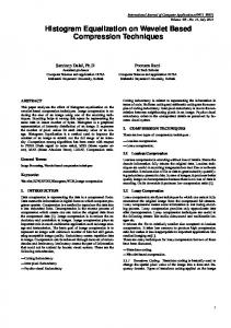
In (6-8), k ∈ [0, K − 1], s ∈ [0, M − 1], and t ∈ [0, L − 1], where K, S, L are the number of discrete levels for each color component cc1 , cc2 , and cc3 , respectively. 3. SMOOTHING The method of histogram equalization presented in (6)-(8) suffers from the sparse data problem which is blamed for the presence of unwanted artifacts in the equalized images. It can be easily seen that working in the color space described above, there are K, K · M and K · M · L possible different color component combinations for (6), (7), and (8), respectively. The observed color component combinations, however, do not exceed the total number of image pixels N and as a result the probabilities of the unseen events are forced to zero. This problem can be visually verified by the presence of “gaps” in the histogram of the equalized image (there are empty bins between very full bins). Fig. 1 depicts the histogram of saturation in an original and an equalized image by the Adobe Photoshop procedure for simplicity reasons. 4000
8000
3500
7000
3000
6000
2500
5000
2000
4000
1500
3000
1000
2000 1000
500 0
(4)
t
frequency
where k ∈ [0, L − 1] represents a grey level, Nk is the number of occurrences of the gray level k and N is the total number of pixels in the image. The transformation function T applied to image I for a given grey level k results in:
=
ycc3 ,t
frequency
The histogram equalization technique for gray scale images attempts to uniformly distribute the pixels of an image I to all the available gray levels L. That is, if the original pixel distribution is F a transformation function T ()has to be defined such that T (F) � U, where U is the uniform distribution. Assuming indexes i, j that run over the image, the normalized image histogram is described by: � � N f (k) = P I(i, j) = k = k (1) N
P(xcc1 = k, xcc2 = m) P(xcc1 = k) m=0 s
∑
0
50
100 150 saturation level
a
200
250
0
0
50
100 150 saturation level
200
250
b
Figure 1: Histograms of saturation for (a) the original and (b) the equalized image by Abode Photoshop. In our approach, to alleviate this problem we used smoothing, a well-known technique, which is largely applied in language modeling for counteracting the effects of statistical variability that turn up in small data sets [15]. Among the various backing-off techniques, such as Good Turing estimates, absolute discounting, linear discounting etc., and the interpolation approaches, such as linear interpolation, which are met in smoothing literature, we selected absolute discounting, a back-off method that amounts in a strict choice between a specific and a generalized distribution. More precisely, since we have three probability distributions to estimate which are interdependent, a multi-level smoothing was conducted in order to recursively smooth the higher order back-off probability distribution by means of the immediate lower order probability distribution. That is, the back-off distribution for the probability (8) is smoothed by the distribution (7), which in turn may be smoothed by the
distribution (6). This process can be described by the following equations:
1800 4000 1600 3500 1400 3000
P(xcc1 = k) =
⎪ ⎪ ⎩
1200
1
= k) > 0
if N(xcc1 = k) = 0
frequency
N(xcc =k)−bcc 1 1 if N(xcc1 N N−n0 1 bcc1 N · ∑ 1 i:N(xcc =i)=0
frequency
⎧ ⎪ ⎪ ⎨
2500 2000 1500
400
500
(9)
P(xcc2 = s|xcc1 = k) = ⎧ N(x =k,x =s)−b cc1 cc2 cc2 ⎪ if N(xcc1 = k, xcc2 = s) > 0 ⎪ ⎪ N(xcc =k) ⎨ 1 N−n0 (xcc =k) P(xcc =s) 1 2 = ⎪ bcc2 N(xcc1 =k) · ∑i:N(xcc =k,xcc =i)=0 P(xcc2 =i) ⎪ ⎪ 1 2 ⎩ if N(xcc1 = k, xcc2 = s) = 0 (10)
800 600
1000
0
1000
200
0
50
100 150 saturation level
200
250
a
0
0
50
100 150 saturation level
200
250
b
Figure 2: Histograms of saturation for (a) the original and (b) the equalized image with smoothed probabilities.
was developed and applied to different color images. The quality of the results was confirmed both from the human visual perspective and objective measures, such as histogram entropy and Kullback-Leibler divergence between the resulted histogram and the uniform one. Initially, the experiments were conducted in the RGB color space. All the probabilities of the form P(xR = k), P(xG = s|xR = k) and P(xB = t|xG = s, xR = k) were estimated P(xcc3 = t|xcc2 = s, xcc1 = k) = according to (9)-(11) and then the transformation functions ⎧ N(xcc =k,xcc =s,xcc =t)−bcc (6)-(8) were calculated. The 3-D histogram of the equalized 1 2 3 3 ⎪ ⎪ N(xcc =k,xcc =s) image proved to be uniform, but its colors were largely dis⎪ ⎪ 1 2 ⎪ ⎪ torted invoking an unsatisfactory visual perception. This reif N(x = k, x = s, x = t) > 0 ⎪ cc cc cc 1 2 3 ⎪ ⎨ N−n0 (xcc =k,xcc =s) sult validated the inability of the RGB space to handle the 1 2 bcc3 N(xcc =k,xcc =s) = (11) perceptual properties of color (hue, intensity, and saturation) 1 2 ⎪ ⎪ P(xcc =t|xcc =s) ⎪ that is stressed in literature. More precisely, hue that deter⎪ 3 2 ⎪ · ⎪ ∑i:N(x =k,x =s,x =i)=0 P(xcc3 =i|xcc2 =s) mines the kind of color (i.e. red, green) should be left un⎪ cc1 cc2 cc3 ⎪ ⎩ changed in order to avoid the color distortion in images. if N(xcc1 = k, xcc2 = s, xcc3 = t) = 0 Contrary to the RGB space, the components of the HSI space correspond directly to the perceptual attributes of In the just described equations (9)-(11), the following notacolor. This is the reason why the proposed histogram equaltion is used: ization approach was tested on HSI, where only the intensity • n0 is the number of unseen color component values, and saturation components were modified, since hue should • n0 (xcc1 = k): the number of cc2 color component values be left unchanged. That is, the transformation functions yI that are never seen given that the cc1 component value is and yS given yI defined by (6)-(7) were estimated with the k, help of P(xI = k) and P(xS = s|xI = k) by employing (9)• n0 (xcc1 = k, xcc2 = s): the number of cc3 color com(10). The equalization was also tested by reversing the order ponent values that are never seen given that the cc1 of transformations, i.e., by first equalizing with respect to yS component value is k and the cc2 component value is s, and then with respect to yI given yS . The latter transformation yielded visually unsatisfactory results. For this reason, n(3) only the results of the histogram equalization through the • bcc3 = (3) 1 (3) where n +2n modification of the I component and the joint modification 1 2 n(3) of the I and S components are presented in Fig. 3 and Fig. 4. r = ∑i, j,t:N(xcc =i,xcc = j,xcc =t)=r 1 1 2 3 The actual size of the images is larger than that shown. As n(2) it can be easily observed, the equalized images have a better • bcc2 = (2) 1 (2) n +2n contrast and they look more colorful. The only unwanted ar1 2 tifact one can reveal is the presence of the grey color in some where n(2) = 1 ∑ r i, j:N(xcc =i,xcc = j)=r 1 2 very small image regions. n(1) The uniform joint distribution between I and S compo• bcc1 = (1) 1 (1) where n(1) = 1 ∑ r i:N(xcc =i)=r n +2n 1 nents for the original and the equalized images were com1 2 pared by means of the entropy and the Kullback-Leibler diBy applying (9)-(11) to estimate the joint probabilities that vergence. appear in (6)-(8), the zero frequency problem in the resultEntropy which represents the average uncertainty of a ing equalized histogram is prevented. Indeed, by comparing random variable is maximized in the case of uniform disFig. 2b and Fig. 1b, it is seen that the histogram of saturation tribution [16]. The entropy of the bivariate color histogram after having applied smoothing does not suffer from the zero distribution is defined by: frequency problem. 4. EXPERIMENTAL RESULTS
H(xcc1 , xcc2 ) =
The histogram equalization method presented in Section 2 enhanced with smoothing, as it is formulated in Section 3,
−
K−1 M−1
∑ ∑ P(xcc1 = k, xcc2 = s)
k=0 s=0
� � · log2 P(xcc1 = k, xcc2 = s) .
(12)
In Table 1 some representative entropy results are presented for six different images. Besides the color images indexed by 1 and 2, that are depicted in Fig. 3 and Fig. 4 another four color image were employed. The latter images belong to the same set of digitized Greek Orthodox Holy Icons with the image indexed by 2. As it can be easily seen, the equalized images have higher entropy than the corresponding original images, as it was expected. Table 1: Entropy of the bivariate color histogram distribution of the original and the equalized images. Image Index Original Equalized 1 12.388753 13.215272 2 11.951549 13.295968 3 11.876878 13.411052 4 11.939243 13.415663 5 12.001775 13.459489 6 12.689356 13.493082 The Kullback-Leibler divergence measures the difference between two probability distributions [16]. In our experiments, Kullback-Leibler divergence was used in order to measure how similar the histograms of the original and the equalized images are to the uniform distribution. The images probabilities which were taken under consideration were those used for the entropy estimate. That is, D( f (xcc1 , xcc2 )||g(xu , yu )) =
∑ ∑ P(xcc1 = k, xcc2 = s) �
· log2
P(xcc1 = k, xcc2 = s) g(xu , yu )
(b)
(c) Figure 3: (a) Original Image (Image Index 1), (b) Equalized Image with smoothed probabilities, and (c) Equalized Image by Adobe Photoshop.
K−1 M−1 k=0 s=0
(a)
� (13)
where g(xu , yu ) is a two-dimensional uniform distribution defined in the same space with f (xcc1 , xcc2 ). The KullbackLeibler divergence results for the processed images are presented in Table 2. The results demonstrate that the color distribution of the equalized images is more closer to the uniform distribution one than that of the original images. Table 2: Kullback-Leibler divergence for the bivariate histogram for the original and the equalized images. Image Index Original Equalized 1 2.503125 1.930227 2 2.806172 1.874292 3 2.857930 1.794522 4 2.814702 1.791326 5 2.771358 1.760948 6 2.294764 1.737663
be easily extended to color spaces with any number of color components. Moreover, the algorithm is enhanced with better probability estimates by means of multi-level smoothing, thus eliminating the zero-frequency problem which produces unwanted artifacts. The experimental results have shown the efficiency of the algorithm in contrast improvement and colorfulness together with the absence of artifacts observed in the traditional equalization processes. The validity of the visual results was also proved by the estimated values of the entropy and the Kullback-Leibler divergence that were introduced in order to assess the uniform nature of the probability density functions. Acknowledgment This work has been supported by the FP6 European Union Network of Excellence MUSCLE “Multimedia Understanding through Semantics, Computation and LEarning” (FP6507752). REFERENCES
5. CONCLUSIONS
[1] J. M. Soha and A. A. Schwartz, “Multidimensional histogram normalization contrast enhancement,” in Proc. 5th Canadian Symp. Remote Sensing, 1978, pp. 86–93.
Concluding, the presented color histogram equalization tries to exploit the correlation between color components. It can
[2] R. N. Niblack, An Introduction to Digital Image Processing, Prentice-Hall Int., 1986.
ification of 24-bit color images in the color difference (c-y) color space,” J. Electron. Imag., vol. 4, no. 1, pp. 15–22, 1995. [11] L. Lucchese, S. K. Mitra, and J. Mukherjee, “A new algorithm based on saturation and desaturation in the xy-chromaticity diagram for enhancement and re-rendition of color images,” in Proc. IEEE Int. Conf. Image Processing, 2001, pp. 1077– 1080.
(a)
[12] E. Pichon, M. Niethammer, and G. Sapiro, “Color histogram equalization through mesh deformation,” in Proc. IEEE Int. Conf. Image Processing, 2003, vol. 2, pp. 117–120. [13] J. Duan and G. Qiu, “Novel histogram processing for colour image enhancement,” in Proc. IEEE Int. Conf. Image and Graphics, 2004. [14] A. Papoulis, Probability, Random Variables and Stochastic Processes, McGraw Hill, New-York, third edition, 1991.
(b)
(c) Figure 4: (a) Original Image (Image Index 2), (b) Equalized Image with smoothed probabilities, and (c) Equalized Image by Abode Photoshop. [3] I. M. Bockstein, “Color equalization method and its application to color image processing,” J. Opt. Soc. Amer., vol. 3, no. 5, pp. 735–737, 1986. [4] W. F. McDonnel, R. N. Strickland, and C. S. Kim, “Digital color image enhancement based on the saturation component,” Optical Engineering, vol. 26, no. 7, pp. 609–616, 1987. [5] P. E. Trahanias and A. N. Venetsanopoulos, “Color image enhancement through 3-d histogram equalization,” in Proc. 11th IAPR Conf. Pattern Recognition, 1992, vol. III, pp. 545– 548. [6] I. Pitas and P. Kiniklis, “Multichannel techniques in color image enhancement and modeling,” IEEE Trans. Image Processing, vol. 5, no. 1, pp. 168–171, January 1996. [7] P. A. Mlsna and J. J. Rodriguez, “A multivariate contrast enhancement technique for multispectral images,” IEEE Trans. Geosci. Remote Sensing, vol. 33, no. 1, pp. 212–216, 1995. [8] P. A. Mlsna, Q. Zhang, and J. J. Rodriguez, “3-d histogram modification of color images,” in Proc. IEEE Intl. Conf. Image Processing, 1996, vol. III, pp. 1015–1018. [9] Q. Zhang, P. A. Mlsna, and J. J. Rodriguez, “A recursive technique for 3-d histogram enhancement of color images,” in Proc. IEEE Southwest Symp. Image Analysis and Interpretation, 1996, pp. 218–223. [10] A. R.Weeks, G. E. Hague, and H. R. Myler, “Histogram spec-
[15] H. Ney, S. Martin, and F. Wessel, “Statistical language modeling using leaving-one-out,” in Corpus-Based Methods in Language and Speech Processing, (S. Young and G. Bloothooft), Eds., pp. 174–207. Kluwer Academic Publishers, Dordrecht, The Netherlands, 1997. [16] C. D. Manning and H. Schutze, Foundations of Statistical Natural Language Processing, MIT Press, 1999.