197
A Fast Mesh-Growing Algorithm for Manifold Surface Reconstruction Luca Di Angelo1, Paolo Di Stefano2 and Luigi Giaccari3 University of L’Aquila,
[email protected] University of L’Aquila,
[email protected] 3 ANSYS Germany Gmbh,
[email protected] 1
2
ABSTRACT In a previous paper these authors presented a new mesh-growing approach based on the Gabriel 2 – Simplex (G2S) criterion. If compared with the Cocone family and the Ball Pivoting methods, G2S demonstrated to be competitive in terms of tessellation rate, quality of the generated triangles and defectiveness produced when the surface to be reconstructed was locally flat. Nonetheless, its major limitation was that, in the presence of a mesh which was locally non – flat or which was not sufficiently sampled, the method was less robust and holes and non – manifold vertices were generated. In order to overcome these limitations, in this paper, the performance of the G2S meshgrowing method is fully improved in terms of robustness. The performances of the new version of the G2S approach (in the following Robust G2S) has been compared with that of the old one, and that of the Cocone family and the Ball Pivoting methods in the tessellation of some benchmark point clouds and artificially noised test cases. The results obtained show that the use of the Robust G2S is advantageous, as opposed to the other methods here considered, even in the case of noised point clouds. Unlike the other methods, the one which is proposed preserves manifoldness and geometric details of the point cloud to be meshed. Keywords: surface reconstruction, triangular meshes, reverse engineering. DOI: 10.3722/cadaps.2013.197-220 1
INTRODUCTION
The approximation of a 3D surface from its point samples is a very important issue in the scientific and engineering realms. Depending on the application, various formulations to this problem can be furnished with various requirements in the input and the output. Among those formulations, the applications of triangular meshes obtained from scanned point clouds are wide–ranging and include Reverse Engineering, Collaborative Design, Inspection, Computer Vision, Dissemination of Museum artifacts, Medicine, Movie Special Effects, Games and Virtual Worlds. For all the applications, the Computer-Aided Design & Applications, 10(2), 2013, 197-220 © 2013 CAD Solutions, LLC, http://www.cadanda.com
198
meshes obtained must match the original data set in terms of geometric and topological criteria. Those objectives are hard to be achieved since scanned point clouds are typically noisy and badly sampled in some areas difficult to access and they have a non-uniform density. Nowadays, these critical aspects are only partially limited thanks to the introduction of scanning systems which offer high resolutions with a measuring accuracy as high as 10 μm. As a direct result, the necessity to manage very large data sets is becoming even more important. The typical triangulation speed of the methods presented in literature may not be enough for the tessellation of a cloud with over one million points. Furthermore, as regards the defectiveness produced, even the methods which are considered to be very robust can generate non–manifold vertices. It is important to highlight the fact that much of the software used for mesh elaboration may not work in the presence of this type of vertices. These authors have recently proposed a new mesh-growing method based on the Gabriel 2 – Simplex (G2S) criterion. The results obtained are very promising since they demonstrate that this method makes it possible to tessellate quickly clouds with over one million points even by using a laptop. Its major limitation is however that, in the presence of a mesh which is locally non–flat or which is not sufficiently sampled, the method is less robust and therefore holes and non–manifold vertices are generated. We should bear in mind the fact that the mesh may be unusable without the deletion of this kind of vertices, which has to be carried out without compromising the areas which have been correctly reconstructed. In order to overcome these limitations, and as it is going to be shown in this paper, the performance of the G2S mesh-growing method is fully improved in terms of robustness. To this end, an original priority queue for the driving of the front growth and a post-processing to efficiently erase the non–manifold vertices are proposed. The improved method has been tested for the tessellation of some benchmark point clouds and artificially noised test cases. The results derived from these experiments are critically discussed hereinafter. 2
RELATED WORKS
Various algorithms to tessellate point clouds have been proposed throughout literature. Some recent exhaustive overviews are available in [1] and [2]. Surface reconstruction algorithms are generally divided into three categories: · implicit; · Voronoi/Delaunay-based; · mesh growing - based. 2.1
Implicit Methods
In implicit methods the surface reconstruction is obtained by extracting the nominally zero – level set of a properly defined implicit function f(p)=0 (where p is either the whole point cloud or only a part of it), formulated so as to be negative inside the point cloud object and positive outside. Typically, the tessellated surface is obtained by applying the Marching cubes algorithm [3] to the iso-surfaces. The most important methods belonging to this group differ in whether the implicit function is defined: · as the sum of radial basis functions (RBF) centred at the points [4], [5]; · as a set of constraints that force the function and its gradient to assume given values at the sample points (Moving Least Squares) [6], [7], [8]; · as a Poisson problem [9].
Computer-Aided Design & Applications, 10(2), 2013, 197-220 © 2013 CAD Solutions, LLC, http://www.cadanda.com
199
A typical shortcoming of implicit methods is that they are sensitive to the outliers. With a view to overcoming this limitation, some new methods ([10], [11], [12] and [13]), based on stratified reconstruction strategies, have been recently developed. By and large, all these methods, on the one hand, carry out a watertight surface reconstruction even in the case of sparse and noisy data but, on the other hand, require many computations and, sometimes, even the surface normal at each data point. Since the final surface may not pass through all the points, the computational time increases as the fitting accuracy increases. Finally, as pointed out by Yang et al. in [8], the resulting mesh must be further refined and optimised. 2.2
Voronoi/Delaunay-based Methods
This group includes algorithms that compute a volume tetrahedralisation by means of a 3D Delaunay triangulation of the sample points. The most important methods presented in the related literature ([14], [15], [16], [17], [18], [19], [20] and [21]) differ essentially in the way they remove the tetrahedra and build the external triangular mesh. In the Crust method, proposed by Amenta et al. in [14], the set of candidate triangles (called Crust) are those having three vertices which are not poles (for each point p of the cloud the poles are the two Voronoi vertices which are farthest from p). Since the Crust is still not a manifold, in order to extract a topologically correct surface, a walking strategy is employed in candidate triangles. The worst time complexity of the Crust algorithm is Θ(m2), where m is the number of points plus poles. In order to reduce running time and memory consumption, while still providing the same theoretical guarantees, Amenta et al. in [15] proposed an improvement of the Crust algorithm, which they called Cocone. The candidate triangles are those triangles inside the Cocone region, which is the complement of a double cone which has its apex at the point under analysis (p) and an assigned opening angle and whose axis is the normal at p. The Cocone’s worst time complexity is Θ(n2), where n is the number of points. As pointed out by Chang et al. in [2], the theoretical guarantee of obtaining a correct reconstruction with the Crust and Cocone methods is only possible as long as the point cloud is well sampled. Dey and Goswami proposed other Cocone versions, one suited to provide a watertight closed surface reconstruction, which they called Tight Cocone [16] and the other suited for noisy data called Robust Cocone [17]. Dey et al. in [18] proposed the Super Cocone algorithm so as to manage large amounts of data. In that method, the entire set of sample points is partitioned into smaller clusters using an octree subdivision, and the Cocone algorithm is applied to each cluster separately. A further evolution of the Crust is the Power Crust proposed by Amenta et al. in [19]. This algorithm can generate a watertight mesh for any point cloud which is sampled enough but it could be non-manifold. Furthermore, sharp edges or noisy data can result in defectiveness. Gopi et al. in [22] proposed a different approach which, for each sample point, provides the projection of the neighbouring points onto the approximating tangent plane as well as the tessellation of the projections by means of a 2-D Delaunay triangulation. The 2D edges obtained are then applied to 3D space. With a view to enhancing the performance of the Delaunay-based methods, CohenSteiner and Da in [20] proposed the Greedy algorithm, which selects the triangles sequentially. The selection of candidate triangles is carried out by the plausibility grade, which is an empirical function of the circumradius and the dihedral angle between adjacent triangles. As stated by Cazals and Giesen in [23], this method “may fail to interpolate all points or to provide a closed surface essentially due to the presence of slivers”. 2.3
Mesh-growing Methods
In mesh – growing approaches the surface reconstruction starts with a seed triangle and the meshed area is grown by pushing the fronts ahead using some criteria. Bernardini et al. [24] introduced the Ball Pivoting Algorithm (BPA), by which the front grows as a ball of user-defined radius pivots around Computer-Aided Design & Applications, 10(2), 2013, 197-220 © 2013 CAD Solutions, LLC, http://www.cadanda.com
200
the front edge. When the ball touches three points, a new triangle is formed. This method affords a correct triangulation for any uniform data point, also in presence of noise, but it has some difficulties in the tessellation of concave areas with little curvature radius. Huang and Menq in [25] proposed an algorithm which, for each front edge, projects the k-nearest points of two endpoints onto the plane that is defined by the triangle adjacent to the front edge. Any point generating triangles whose edges intersect edges of already-existing triangles is discarded. Of the points which are retained, the point showing the minimum sum of distances from the front-edge endpoints is chosen. Nonetheless, as pointed out by Lin et al. in [26], this algorithm presents some shortcomings. In order to overcome them, Lin et al. in [26] introduced the Intrinsic Property Driven (IPD) algorithm, which improves the way of searching for the points to be triangulated. As stated by Chang et al. in [2], all the methods based on mesh-growing approaches are fast, efficient and simple to implement but they, however, may fall short whenever two surfaces are either close together or near sharp features. More recently, Li et al. in [1] proposed a method based on a Priority Driven approach that evaluates shape changes from an estimation of the original surface that is made at the front of the mesh-growing area. The experimental results in [1] evidenced that the triangulation speed of the method was higher than that of the Ball Pivoting and the Cocone. However, no reckoning was made of the defectiveness generated by the method. Finally, in [27] these authors put forth a new mesh growing approach based on the Gabriel 2 – Simplex (G2S) criterion: A triangle is a G2S if its smallest circumscribing ball is empty. This criterion degenerates into the classical 2D Delaunay if all the points are coplanar. As a direct consequence, the flatter the surface appears to be locally, the better is the guarantee of a good reconstruction. More generally, the theoretical guarantee of a good reconstruction can be founded on the following theorem demonstrated by Dyer et al. in [29]: A Gabriel mesh is a Delaunay mesh. In other words, any mesh in which every triangle verifies the G2S criterion verifies also the 3D Delaunay one. As opposed to the 2D and 3D classical Delaunay criterion, for a given data set, the G2S triangulation is not unique and depends on the chosen seed triangle. The G2S criterion has already been used in some tessellation methods presented in literature. Ruiz et al. in [30] used it as a basis for a method for parametric surface meshing. This method cannot be used directly for the triangulation of point clouds since it is based on information such as the pre-image in a parametric space, the boundary, and local curvatures. Cohen-Steiner and Da in [20] and Ma et al. in [21] used the G2S criterion in order to select the external triangular facets of tetrahedra coming from a 3D Delaunay triangulation. The method proposed by Di Angelo et al. in [27] applied the G2S criterion directly to a point cloud so as to identify triangles pertaining to the external surface. This method has proven to be competitive in terms of tessellation rate, quality of the generated triangles and defectiveness produced when the surface to be reconstructed is locally flat. Nonetheless, in the presence of a noisy mesh or a mesh which is locally non–flat or which is not sufficiently sampled, the method generates defectiveness such as holes and non–manifold vertices. 3
THE GABRIEL 2 – SIMPLEX CRITERION BASED METHOD
The mesh-growing method proposed in [27] consists of the following steps: step 1. Import of the point cloud; step 2. Building of a specific data structure to speed up the search for the nearest point; step 3. Search for the seed triangle; step 4. Surface triangulation. The first step involves importing the point cloud which pertains to a continuous surface in the form of the coordinates x, y, z. Other information, such as the normal at points, is not required. All the points from the cloud are held in an original hash table data structure, applied to an improvement Computer-Aided Design & Applications, 10(2), 2013, 197-220 © 2013 CAD Solutions, LLC, http://www.cadanda.com
201
of the typical space division approach ([31] and [32]), which makes it possible a more efficient search for the nearest neighbourhoods. Then, the seed triangle is selected by using a new approach which guarantees that it pertains to smooth features of the external surface of the point cloud. Starting from the seed triangle, the meshed area grows, coherently with a manifold surface, by pushing the fronts ahead using the G2S criterion. 3.1
Selection of the Seed Triangle
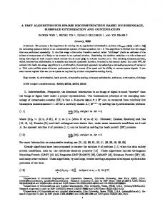
The G2S criterion being applied does not ensure that the triangles belong to the external surface. In fact, the G2S triangles can either lie on the external surface or be transversal to it. Thus, as it happens with the other mesh-growing approaches, the selection of the seed triangle is an important aspect of the proposed method. The seed triangle is selected based on an original strategy consisting of the following sub-steps: Step 3.1. A point of the cloud is randomly chosen. Step 3.2. Its nearest neighbour point is searched for, and an edge is formed between these two points. Step 3.3. The third point of the triangle is searched for within a sphere centred at the midpoint of the edge and whose radius is k-times the length of the edge (k can be either a user-defined parameter or a default value). Step 3.4. Each point in the range is connected to the edge in order to form a triangle. Step 3.5. Selection of the seed triangle. The seed triangle verifies the G2S criterion and the points contained in the infinite cylinder passing through its three vertices, and having the axis parallel to its normal, are all above or all under the triangle (figure 1). The procedure is repeated until a triangle, satisfying the conditions in step 3.5 is found. The cylinder test also excludes any G2S triangles which are in correspondence of sharp points. 3.2
G2S Criterion-based Triangulation
The edges of the seed triangle constitute the initial advancing front of the growing-mesh method. For each free edge (ef) (which are edges pertaining to only one triangle) of the growing front a triangle is generated according to the following procedure sub-steps: Step 4.1: Identification of all the candidate points near ef. Typically, the reference point is chosen among the candidate points, which are those inside a properly defined search region. In this paper the search region is a sphere having its centre (search region centre) lying on the plane of the front triangle on the axis of the free edge under analysis in the growing direction, and having the search radius as radius (figure 2). The search radius value affects tessellation quality and time. A low search radius keeps the search region near the front edge, so the method falls short in the meshing of under sampled areas. A high search radius, on the other hand, reduces the tessellation rate and sometimes generates defectiveness. An automatic approach has been implemented to set the search radius value. It changes the search radius value from an initial value (in the following test cases it is equal to the length of the free edge under analysis) to an assigned maximum value according to a given step value. The search radius is increased up to the maximum value if no points are found inside the search region. Since the search region centre lies on the same plane as the front triangle, the search method usually favours finding candidate points in the area wherein the surface is expected to grow. In typical practical situations, this prevents further controls that may cause the algorithm to slacken. Furthermore, this search region excludes from candidate points those points which are farther away or those points which could generate thin and slivery triangles. Finally, this criterion generally stops the front in the presence of sharp edges. Computer-Aided Design & Applications, 10(2), 2013, 197-220 © 2013 CAD Solutions, LLC, http://www.cadanda.com
202
The triangle is not a good seed triangle
The triangle is a good seed triangle
Fig. 1: The cylinder test to select a seed triangle. Step 4.2: Selection of the reference point in the search region. When more than one point is found inside the search region (cp1, cp2 and cp3 in figure 3a), for each point the smallest sphere passing through it and the front edge’s points is traced. The point which verifies the G2S triangle is the candidate point. Then, the candidate triangle (figure 3b) is submitted to topological tests. In order to speed up the triangulation process, if only one point is found inside the search region, that point is directly assumed to identify a candidate triangle with the free edge (ef) without verifying whether or not it is a G2S. For a quasi–locally flat point cloud, the candidate triangle has a high probability of being G2S. Finally, if no point is found inside the search region, ef is removed from the free edges’ queue and it is classified as boundary edge. Step 4.3: Topological tests and algorithm control. Each of the new triangles retained is formed by the front edge (ef) and two further edges (e1 and e2). In order to check efficiently whether these two edges (e1 and e2) are really new or they already belong to other triangles, a data structure called Point Edge Map (PEM) is proposed which relates every point to its edges. For either edge (e1 and e2), the following conditions should be verified: -
If the edge already pertains to another triangle, the consistency of the orientation of the new triangle with the triangle sharing the edge must be verified.
-
If this edge is new, it is added to the Point Edge Map and to the front queue and ef is removed from the front queue. The procedure ends when the free edges’ queue is empty.
Computer-Aided Design & Applications, 10(2), 2013, 197-220 © 2013 CAD Solutions, LLC, http://www.cadanda.com
203
Extreme points of the free edge under analysis Candidate points Outer points
Search region
free edge under analysis
Search region centre Search region radius Front triangle
Fig. 2: The search region’s definition terms.
Search region
free edge under analysis cp1
cp2 cp3
Search region centre Search region radius
candidate triangle
cp1
cp2
Front triangle cp3 a) b)
Fig. 3: Reference point selection.
3.3
Some Considerations
The theoretical basis of G2S is taken for granted by accepting the fact that point clouds can be considered locally flat, or, in other words, that the surface to be reconstructed is locally oriented, smooth, manifold, well sampled and not self-intersecting. Under this hypothesis, the G2S criterion works like a 2D Delaunay tessellation through which surface reconstruction is guaranteed. These requirements are not so restrictive anymore, especially since the advent of high-resolution non– contact scanners which produce noise-free points clouds. More generally, as pointed out by Dyer et al. in [29], a Gabriel mesh (a mesh for which each triangle verifies the G2S criterion) is a Delaunay mesh. In [27] these authors already demonstrated it by analysing the typical benchmarks presented in the related literature: -
the triangulation speed of G2S is comparable with a traditional 2D Delaunay-based mesher and it is at least an order of magnitude higher than the other methods here considered; Computer-Aided Design & Applications, 10(2), 2013, 197-220 © 2013 CAD Solutions, LLC, http://www.cadanda.com
204
-
G2S produces triangles whose quality is similar to that of those triangles obtained by the Cocone methods and slightly better than the quality of the triangles obtained by the Ball Pivoting one;
-
G2S can reproduce even the smallest details of well sampled surfaces, similarly to Cocone methods, also in concave areas of strongly non–uniform point clouds where the Ball Pivoting method shows some problems;
-
G2S does not produce non–manifold edges, self-intersecting triangles or slivers;
-
as regards non–manifold vertices, holes and boundary edges, the quantity and the extension of defectiveness generated by the G2S tessellation are on average similar to those produced by the Cocone and the Tight Cocone;
-
in the presence of a mesh which is locally non–flat or which is not sufficiently sampled, G2S is less robust and holes and non–manifold vertices are generated.
4
CRITICAL ASPECTS IN THE G2S METHOD AND IMPROVEMENTS
As mentioned in the previous section, the G2S version proposed in [27] presents some critical aspects. In particular, in any area of a point cloud that is not locally flat or is not sufficiently sampled, G2S can generate: -
holes, which identify unmeshed area;
-
a twisting of the surface;
-
non–manifold vertices.
In order to eliminate non-manifold vertices, in literature some methods are proposed ([33] and [34]). Typically, these methods work as a step that is completely independent from the tessellation phase, by using static large data structures which could be inadequate to repair meshes with some millions of triangles. This paper focuses on the improvement of the G2S performance as regards the generation of twisted surfaces and non–manifold vertices. The methods here proposed take advance from the data generated by the mesh growing algorithm and they can manage millions of triangles. 4.1
The Twisting of the Surface
In this paper, the twisting of the surface identifies the generation on the same body of different tessellated surfaces not having congruent normal (figure 4). This in turn generates holes with extended boundary edges since adjacent patches not having a congruent orientation cannot be merged. In order to solve this problem, an original priority queue is proposed. The main idea at the basis of the priority approach being presented is to mesh first those areas for which the front grows in the flattest way in the neighbourhood.
Fig. 4: The twisting of the surface.
Computer-Aided Design & Applications, 10(2), 2013, 197-220 © 2013 CAD Solutions, LLC, http://www.cadanda.com
205
In order to speed up the algorithm, a set of discrete values is adopted for a priority index. The strategy used involves the definition of: -
n priority levels for the search neighbourhood dimension, so that the smallest dimension has priority pld = 1 and the greatest has priority pld = n);
-
m priority levels for flatness, measured as the angle (β) between the normal of the triangle containing the free edge under analysis (front triangle) and the candidate triangle (priority plf = 1 being assigned to β=0° and priority plf = m to β=180°).
The priority index (PI) is defined according to the following expression: PI = m ·( pld – 1) + plf
(4.1)
Next, these edges are positioned in the queue by sorting, in ascending order, the value of PV calculated for the corresponding candidate triangle. 4.2
Non – manifold Vertices Elimination
In what follows, the triangles with at least one boundary edge are referred to as boundary triangles and the vertices, for which the incident triangles form more than one fan are referred to as non-manifold vertices. In this paper the two common types of non-manifold vertices, reported in the figure 5, are considered. In order to verify that a vertex is manifold, the sequence of triangles sharing the vertex is analysed. For this purpose, a specific data structure has been defined; -
a dynamic queue of edges (deq) containing the non-analysed edges which initially has ne rows (ne is the number of edges that are not boundary) and six columns: the edge label (el), its extreme points (pf and pl) and the triangles sharing the edge tf and tl);
-
a nv·4 matrix (ptt) (nv is the number of vertices); in each row of ppt the sequence of adjacent triangles sharing the vertex (vl) is represented by storing the first (front) and the last (back) triangle of the sequence and the number of the triangles found (nt,a). A vertex is checked to be manifold if nt,a is equal to the number of triangles sharing the vertex.
v v a)
b)
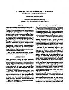
Fig. 5: Common types of non – manifold vertices. In order to explain this method, let us consider the mesh represented in figure 6a with the labels of the vertices, edges and triangles superimposed. First, the deq is filled with the edges of the mesh, except for the boundary ones (figure 6b) and in the ptt table, the labels of all vertices are added to the first column (figure 6c). The process starts by popping the first element off the queue (e3) and the corresponding labels of tf (t1) and tl (t 2) are added to the related lines of the matrix (figure 6d). Then, the first element of the new queue (figure 6e) is popped off (e6). Since the triangles’ labels associated with v1 for e6 (t3 and t8) are different from those reported in the corresponding row of the matrix, this edge is pushed to the end of the queue (figure 6f). If once the queue has been scanned through, no edges of intersection of one of two extreme triangles of the loop (t1 and t2) have been found for the Computer-Aided Design & Applications, 10(2), 2013, 197-220 © 2013 CAD Solutions, LLC, http://www.cadanda.com
206
vertex under examination (v1), the loop is defined as open since tf ≠ tl. In the case that there are other edges incident to v1 in the queue, the front and back columns of the ptt are emptied (figure 6g). Again, the first element of the queue is popped off (e8); the triangles t1 and t6 are added to the corresponding rows of the matrix of the vertices v1 and v6 (figure 6h). Once more, the first element of the new queue (figure 6i) is popped off (e9). Since one of the two triangles incident to the edge (t 4) is a terminal point (front) of the loop, in the corresponding row of ptt, this triangle is substituted with the other (t3) (figure 6l). This procedure is iterated until the triangles of the front and the back column are the same for a vertex (figure 6m), or, in other words, the loop is closed. In the case that in the deq there are edges incident to that vertex (figure 6n), the corresponding triangles are erased (figure 6o). The procedure ends when the deq is empty. 5
EXPERIMENTAL RESULTS AND DISCUSSION
The methodology described in the previous sections has been implemented in original software, coded in C++. The method being proposed has been tested for the tessellation of several scanned point clouds characterised by different value and uniformity in sampling rate, geometries, topologies and noise level. Most of the test cases used are typical benchmarks taken from the related literature, although some others are artificially noised test cases purposely designed. All the tests have been run on a laptop with 1.86 GHz Intel Pentium M Processor and 1 GB RAM. The performance of the algorithm has been assessed in terms of the tessellation rate ([ktriangles/s]) and the quality of the generated mesh. The latter has been analysed by evaluating: The mean value of the following quality factor of the generated triangles [35]: 3
12 QF = d
Õ (p - d ) i =1
i
(5.1)
p
where di is the length of the i-th side of the triangle, d = max (di ) and p = i = 1,2,3
-
-
3
åd i =1
i
2 . The value of
QF varies from 0 (for triangles having null area) to 1 (for equilateral triangles). This factor is very significant since uniform meshes characterised by equilateral triangles are required in most of the practical uses of tessellated surfaces. The mean value of the distance (μd%) of the unmeshed points from the tessellated surface, normalised on the mean spacing of the point cloud. Since the data points lie on the original surface and outliers are excluded, this index is an estimation of the error in meshing data points. The number of the following defects: § non–manifold vertices (nnmv); § non–manifold edges (nnme); § holes (nholes): unmeshed areas; § boundary edges (nbe): edges bordering the holes.
The performance of the Robust G2S method is compared with that of the old one [27] (henceforth G2S_old) that of the Cocone methods (Cocone [15], Tight Cocone [16] and Robust Cocone [17]), whose implemented software has been kindly provided by the authors, and is also compared with our implementation of the Ball Pivoting [24]. The last two methods can be considered to be reference implementations of the Delaunay tessellation and of the mesh-growing approaches. In the following experiment the closed point clouds are analysed with the Tight Cocone, the open point clouds with the Cocone method and the noisy ones are tessellated by using the Robust Cocone. Neither the G2Ss nor Computer-Aided Design & Applications, 10(2), 2013, 197-220 © 2013 CAD Solutions, LLC, http://www.cadanda.com
207
the Cocone family methods require any empirical input parameters. On the contrary, the BPA needs the ball pivoting radius. The Ball Pivoting performance is largely affected by the setting parameters which must be accurately defined to obtain satisfactory results but a tedious and time-consuming trial–and-error process is required. 5.1
Typical Benchmarks
The first set of experiments consists of the typical benchmarks used in the related literature to evaluate tessellation methods. In particular, 16 closed point clouds and 10 open point clouds, all of them having different geometries and having been scanned with different technologies, are considered. Eight of these point clouds have more than one million points and can be considered to be very large data sets. Figure 7 illustrates renderings of some test cases tessellated with the proposed method. The testing results are reported in table 1 – 6. Some of the benchmark test cases (Neptune, Asian Dragon, Amphora and Thai Statue) cannot be tested with the available Cocone and Tight Cocone implementations which cannot work for them. When analysing the results obtained, it is easy to conclude that all the methods here considered fall short for point clouds (Toywheel, Turtle and Galaad) characterised by a strongly non–uniform sampling. The improvements introduced in Robust G2S, are achieved by a small reduction of the tessellation rate respect to the G2S_old. However, Robust G2S yields results which are, on average, about 300 times and 8 times higher than the Cocone and the BPA methods, respectively. Our implementation of the BPA shows a tessellation rate comparable with the implementation proposed in literature. If we analyse the values for the QF index, the Robust G2S method is verified to produce triangles whose quality is similar (99.58%) to those obtained with the Cocone methods and slightly better than those obtained by means of the Ball Pivoting one (95.29%). Generally speaking, the Robust G2S method (μd%=0.65%) and the Cocone methods (μd%=0.57%) can reproduce even the smallest details of well-sampled surfaces. On the contrary, and owing to difficulties in tessellating concave areas of point clouds, the BPA method produces many unmeshed points (μd%=21.45%). Figure 8 shows the maps of the μd% of the Chinese_Dragon. The Robust G2S reconstructs better the concave areas since, unlike the BPA, the ball radius is locally adapted to point spacing. For all the cases analysed, the Robust G2S does not produce, as opposed to the other methods, non – manifold vertices. Furthermore, when using the priority queue in the new version of G2S, in most cases there is a reduction of holes and boundary edges. In some cases, such as the raptor, the marked reduction in boundary edges is due to the elimination of the problem of twisting surface generation. Figure 9 shows the renderings of the tessellation obtained for the Raptor with both the G2S_old (a) and Robust G2S. In the same figure, the outside of triangles is coloured blue whereas the inside is coloured yellow. The Robust G2S performance is comparable with that of the Cocone family methods which are based on the Delaunay triangulation method, which is intrinsically more robust, but 300 times slower. The Robust G2S method generates defectiveness, essentially in those areas of the point clouds which cannot be considered to be locally flat since the sampling density is not accurate enough to reproduce surface details. 5.2
Noisy Point Clouds
In order to verify the performance of the Robust G2S in the tessellation of noised point cloud data, specific experiments are carried out. The performance of Robust G2S is compared with those of the G2S_old [27], Robust Cocone [17] and the Ball Pivoting [24]. Computer-Aided Design & Applications, 10(2), 2013, 197-220 © 2013 CAD Solutions, LLC, http://www.cadanda.com
208
The first experiment aims at comparing the four methods as regards the tessellation of the Stanford Bunny with different levels of noise added. Noise is randomly generated according to a Gaussian probability density distribution with different values of standard deviation expressed as percentage of the mean spacing of the original point cloud (σ%). Figure 10 illustrates the results of the renderings and table 7 reports the number of defects. In all the cases analysed, the Robust G2S method proves to be capable of reproducing even the smallest details of the model preventing non-manifold edges and vertices. On the contrary, the Robust Cocone and the BPA methods bring about a coarse reconstruction of the model and some important details are completely neglected. It is the case of the Bunny Stanford neck. For a high value of σ% (σ%>25%), the Robust G2S produces a tessellation with a high number of holes and boundary edges. Large random errors being applied to the original model destroy, depending on the ratio between error and point spacing, the characteristic regularity of the original surface to the extent it produces geometric nonsense. In these cases, the assumption of local flatness, which is basic to recognising the nature of a regular surface in a point cloud, is no longer valid. The second set of experiments is carried out in order to compare the four methods as regards the tessellation of the point cloud with different number of outliers. For this purpose, in the Stanford Bunny outliers are randomly added according to the following percentages of the total number of points: 5%, 10% and 20%. The Robust Cocone seems to be inadequate to tessellate point clouds with this type of noise (figure 11). Due to the use of a relatively large ball, the BPA does not process as outliers any points which are external to the regular surface and produce the typical cones shown in figure 11. All in all, the Robust G2S shows good results thanks to the intrinsic characteristic of the method which tends to search for candidate points mainly in the regular growth of the surface. Furthermore, the Robust G2S does not generate non-manifold vertices (table 8) and the number of holes and boundary edges is similar to those produced by the BPA method. 6
CONCLUSION
In a previous paper [27] these authors had already presented a new-mesh growing approach based on the Gabriel 2 – Simplex (G2S) criterion. The results obtained proved that the G2S is competitive in terms of tessellation rate, quality of the generated triangles and low defectiveness, especially when compared with the Cocone family and the Ball Pivoting methods. Its major limitation was that, in the presence of a mesh which was locally non – flat or was not sufficiently sampled, it proved to be less robust and holes and non – manifold vertices were generated. In order to improve the robustness of the G2S mesh-growing method, this paper proposes an original priority queue for the driving of the front growth and a post processing to efficiently erase the non – manifold vertices. The performance of Robust G2S has been compared with that of G2S_old, and that of the Cocone family and the Ball Pivoting methods in the tessellation of some benchmark point clouds and artificially noised test cases. The results derived from these experiments show that the improvements proposed and implemented prevent the generation of non – manifold vertices and make the Robust G2S more robust than G2S_old in terms of generation of defects such as holes and boundary edges, also in presence of noised point clouds. This performance improvement is achieved by a small reduction of the tessellation rate respect to the G2S_old method. However, the tessellation rate is still at least an order of magnitude higher than the Cocone family and the Ball Pivoting methods In the case of much noised meshes, Robust G2S produces more holes and boundary edges than the Robust Cocone and the Ball Pivoting methods, but the last named ones do not preserve important details of the object. Finally, in the presence of meshes with outliers, the number of holes and boundary edges produced by Robust G2S can be said to be comparable with those produced by the Ball Pivoting method. Computer-Aided Design & Applications, 10(2), 2013, 197-220 © 2013 CAD Solutions, LLC, http://www.cadanda.com
209
v3
e4
v4
e2 t2
e3
e5
e11
v9
v6
e10
t5 e12
e8 t6
e14
t4
e7
t3
v5
e6 t8
e15
t7
e12 e13 e15 e18
v7
e9 v1
e8 e9
v2
t1 e1
e13
ptt vl front back v1 v2 v3 v4 v5 v6 v7 v8 v9 v10 v11 v12 v13
deq el e3 e6
e17
pf
pl
tf
tl
v1
v3 v5 v6
t1
t2
t3 t4
t8 t5
v1 v7 v1 v9 v1 v8 v1 v10
t3 t5 t6 t7
v1
t9
t4 t6 t7 t8 t10
v1 v1
v12
b)
e16
v8
v10
c) e20
e21
v11
a)
t9
vl front back v1 v2 v3
v12
e22
deq el e6 e8 e9 e12 e13 e15 e18
pf
pl
tf
tl
v1
v5 v6
t3
t8
t4 t3 t5 t6 t7 t9
t5 t4 t6 t7 t8 t10
v1 v1 v7 v1 v9 v1 v8 v1 v10 v1 v12
el e8 e9
tf
tl
v1
t4
t5
t3 t5 t6 t7
t4 t6 t7 t8 t10
v1 v1 v1 v1 v1 v1
e12 e13 e15 e18 e6
v6 v7 v9 v8 v10 v12 v5
t9 t3
ptt vl front back v1 t4 t5 v2 v3 v4 v5 v6 v7 v8 v9 v10 v11 v12 v13
t5
t4
nt,a 2
el e9
0 0 0
e12 e13 e15 e18 e6
0 2 0 0 0 0 0 0
deq pf pl v1 v1 v1 v1 v1 v1
v7 v9 v8 v10 v12 v5
tf
tl t4 t6 t7 t8 t10
0 0 0 0
v9
e11
2 0 2 0 0 0 0 0 0 0 0 0 0
v7
e10 t4
e8
t5
e12
e9
t7
v8 e20 t9 e21
e7 e6
t3
v1
t6 e13
e14
0 0
t8
e15 e16
v5
e17
v10
e18 e19 t10 v12 e 22
v11
g)
0
v13 ptt
ptt vl front back v1 t3 t5 v2
t3 t5 t6 t7 t9 t3
0 0 0
0 0 0
t8
f)
e)
h)
deq pf pl
0 0 0 0
nt,a
d) nt,a 0 0 0 0 0 0 0
v4 v5 v6 v7 v8 v9 v10 v11 v12 v13
v13
0 0
v6
ptt
e19
e18 t10
ptt vl front back v1 t1 t2 v2 v3 t2 t1 v4 v5 v6 v7 v8 v9 v10 v11 v12 v13
nt,a
t8
i) l)
v3 v4 v5 v6 v7 v8 v9 v10 v11 v12 v13
t5
t4
vl front back v1 t3 t3 v2 v3
nt,a 3 0 0 0 0 2 0 0 0 0 0 0 0
m)
0
v4 v5 v6 v7 v8 v9 v10 v11 v12 v13
t5 t7 t9 v6
e11 v9
o)
t3 t5 t3 t6
e14
t8 t4 t4 t7 t6 t8 t10
nt,a 6 0 0 0 2 2 2 2 2 2 0 2
deq el
pf
pl
tf
tl
e18
v1
v12
t9
t10
n)
0
e10
t5 e12
e8 t6
v8
v7
t4
e13
e9 v1 t7
e15 e16
e7
t3 e6
v5
t8
e17 v10
Fig. 6: Explanation of the post processing used to erase the non – manifold vertices. Computer-Aided Design & Applications, 10(2), 2013, 197-220 © 2013 CAD Solutions, LLC, http://www.cadanda.com
210
a)
b)
d) c)
e) f)
Fig. 7: Rendering of the following test cases: a) Red_circular_box; b) Raptor; c) Oil_pump; d) Turbine_blade2; e) Hand; f) Thai Statue. Computer-Aided Design & Applications, 10(2), 2013, 197-220 © 2013 CAD Solutions, LLC, http://www.cadanda.com
211 Robust G2S No. of No. of Rate Name points triangles [ktriangles/s] Rocker-arm (**) 10,044 20,084 320.9 Stanford Bunny (*) 35,947 71,873 294.3 Horse (**) 48,485 96,873 307.6 Armadillo (*) 172,975 345,897 303.0 ** Pulley ( ) 293,672 587,266 328.5 Hand (**) 327,323 649,768 292.3 Turbine Blade 2 (****) 396,104 791,916 288.5 Dragon (***) 435,545 834,771 304.5 ** Bimba ( ) 502,694 1,005,246 366.2 Happy Buddha (***) 543,652 1,038,953 338.0 Chinese Dragon (**) 655,980 1,311,307 322.0 Red_circular_box (**) 701,322 1,401,530 243.7 *** Turbine Blade ( ) 882,954 1,740,362 351.9 Raptor (**) 1,000,080 1,685,915 349.6 Neptune (**) 2,003,933 4,007,522 261.8 Asian Dragon (*) 3,609,601 7,217,980 362.9 * ( ) http://www.graphics.stanford.edu/data/3Dscanrep/ (**) http://shapes.aimatshape.net/ (***) http://www.lodbook.com/models/ (****) http://www.scansystems.it
G2S_old [27] No. of Rate triangles [ktriangles/s] 20,084 380.1 71,884 321.7 96,859 377.4 345,934 372.8 587,181 371.8 649,527 376.6 792,041 377.3 805,376 348.1 1,005,172 432.5 1,004,540 351.0 1,311,296 475.2 1,400,720 369.5 1,759,357 364.4 1,716,226 439.6 4,007,628 362.8 7,218,442 418.8
Tight Cocone [16] No. of Rate triangles [ktriangles/s] 20,088 1.33 71,884 0.99 96,922 0.82 345,944 0.85 587,312 0.67 654,550 0.67 791,873 1.72 867,282 0.62 1,005,088 0.82 1,081,232 0.51 1,310,435 0.99 1,401,725 0.78 1,759,514 1.11 1,854,921 0.28 -----
Ball Pivoting [24] No. of Rate triangles [ktriangles/s] 18,848 26.18 67,449 22.86 94,382 48.15 307,286 33.18 571,738 52.82 554,266 23.89 736,685 43.69 782,185 35.46 953,618 23.82 809,539 25.36 966,266 25.28 1,367,913 51.15 1,630,254 47.28 1,378,599 43.48 3,119,149 20.01 6,715,376 26.22
Tab. 1: Comparison between the performance of Robust G2S, G2S_old [27], Tight Cocone [16] and Ball Pivoting [24] in closed surfaces.
Computer-Aided Design & Applications, 10(2), 2013, 197-220 © 2013 CAD Solutions, LLC, http://www.cadanda.com
212
Name Rocker-arm Stanford Bunny Horse Armadillo Pulley Hand Turbine Blade 2 Dragon Bimba Happy Buddha Chinese Dragon Red_circular_box Turbine Blade Raptor Neptune Asian Dragon
Robust G2S QF [26] μd % 0.699 1.40∗10−2% 0.708 0.007% 0.714 0.51 % 0.768 0.000% 0.776 5.39*10−3% 0.648 0.005% 0.753 0.06% 0.642 1.63% 0.751 0.005% 0.613 0.145 % 0.771 0.027% 0.785 0.038% 0.585 0.68% 0.723 11.52% 0.765 0.008% 0.903 0.012%
G2S_old [27] QF [26] μd % 1.40∗10−2% 0.699 0.708 0.007% 0.714 0.51 % 0.768 0.000% 0.776 5.39*10−3% 0.648 0.005% 0.753 0.06% 0.642 1.83% 0.751 0.194 % 0.613 0.145 % 0.771 0.027 % 0.785 0.038% 0.585 0.68 % 0.723 17.75% 0.765 0.008% 0.903 0.012%
Tight Cocone [16] QF [26] μd % 0.707 0,000% 0.713 0,029% 0.714 0,42% 0.775 0,005% 0.776 0,085% 0.713 0,009% 0.753 0,108% 0.622 0,819% 0.751 0,322% 0.614 1,39% 0.769 0,208% 0.783 0,053% 0.580 0,553% 0.704 7,345% -----
Ball Pivoting [24] QF [26] μd % 0.651 5.46% 0.675 4.45% 0.695 1.12% 0.708 6.97% 0.761 3.77% 0.620 180.0% 0.698 1.68% 0.611 37.28% 0.590 5.53% 0.734 32.49% 0.673 32.33% 0.765 1.037% 0.580 70.01% 0,663 29.26% 0.749 46.12% 0.887 7.81%
Tab. 2: Comparison between the quality reconstruction of Robust G2S, G2S_old [27], Tight Cocone [16] and Ball Pivoting [24] in closed surfaces.
Computer-Aided Design & Applications, 10(2), 2013, 197-220 © 2013 CAD Solutions, LLC, http://www.cadanda.com
213
Robust G2S holes Model name nnmv nnme nho nbe Rocker-arm 0 0 0 -Stanford Bunny 0 0 0 -Horse 0 0 7 83 Armadillo 0 0 0 -Pulley 0 0 1 4 Hand 0 0 13 90 Turbine Blade 2 0 0 2 9 Dragon 0 0 40 579 Bimba 0 0 6 117 Happy Buddha 0 0 54 508 Chinese Dragon 0 0 19 103 Red_circular_box 0 0 97 635 Turbine Blade 0 0 164 2089 Raptor 0 0 36 207 Neptune 0 0 4 34 Asian Dragon 0 0 31 193
nnmv 0 0 0 0 0 0 0 0 0 0 0 0 0 0 0 0
G2S_old [27] holes nnme nho nbe 0 0 -0 0 -0 8 149 0 0 -1 2 10 0 19 126 10 12 77 1 28 249 11 12 220 32 47 462 47 35 928 27 42 327 42 66 1054 269 91 1508 13 19 107 41 88 721
Tight Cocone [16] Ball Pivoting [24] holes holes nnmv nnme nho nbe nnmv nnme nho nbe 0 0 0 -2 0 5 54 0 0 0 -1 0 0 0 0 0 1 4 11 0 6 111 0 0 0 -0 0 4 16 0 0 0 -0 0 0 -8 0 6 58 0 0 32 186 1 0 1 11 0 0 1 3 23 0 24 166 2 0 31 115 8 0 5 54 0 0 0 -39 0 11 93 0 0 8 41 18 0 13 119 0 0 12 40 12 0 10 75 53 0 501 6538 295 0 109 864 3 0 49 180 7751 0 4335 34781 0 0 7 37 ----0 0 7 37 ----0 0 7 92
Tab. 3: Comparison between the defectiveness produced by Robust G2S, G2S_old [27], Tight Cocone [16] and Ball Pivoting [24] in closed surfaces.
Computer-Aided Design & Applications, 10(2), 2013, 197-220 © 2013 CAD Solutions, LLC, http://www.cadanda.com
214 No. of points 10,010 549,007 596,903 675,049
Robust G2S No. of Rate triangles [ktriangles/s] 19,970 310.8 1,096,742 322.5 1,190,806 319.7 1,349,076 299.7
Name Foot (**) Support (*) Rolling Stage (**) Body (****) Nicolò da 946,760 1,891,949 Uzzano (**) 367.0 Toy wheel (**) 1,001,231 --Amphora (**) 1,317,152 2,590,549 274.6 Galaad (**) 1,451,502 --** Toy turtle ( ) 1,472,131 --Thai Statue (*) 4,999,997 9,994,088 275.1 (*) http://www.graphics.stanford.edu/data/3Dscanrep/ (**) http://shapes.aimatshape.net/ (***) http://www.lodbook.com/models/ (****) http://www.scansystems.it
G2S_old [27] No. of Rate triangles [ktriangles/s] 19,972 352.9 1,097,412 397.6 1,193,303 373.5 1,349,609 279.7 1,891,992 -2,616,596 --9,994,088
464.5 -295.9 --303.8
Tight Cocone [16] No. of Rate triangles [ktriangles/s] 19,982 2.25 1,097,538 1.82 1,193,688 1.49 1,344,039 1.2 1,891,669 1.93
Ball Pivoting [24] No. of Rate triangles [ktriangles/s] 18,332 37.05 1,074,677 49.65 1,168,744 57.07 1,326,963 59.47 1,795,917 40.33
1,702,234 -2,215,146 2,226,103 --
959,810 2,544,331 272,561 670,035 8,335,937
0.41 -0.53 0.60 --
0.27 62.67 0.47 0,53 19.48
Tab. 4: Comparison between the performance of Robust G2S, G2S_old [27], Tight Cocone [16] and Ball Pivoting [24] in open surfaces. Name Foot Support Rolling Stage Body Nicolò da Uzzano Toy wheel Amphora Galaad
Robust G2S QF [26] μd % 0.699 0.000% 0.730 0.237% 0.616 0.006% 0.760 0.250% 0.747 -0.614 --
0.007% -0.004% --
G2S_old [27] QF [26] μd % 0.699 0.000% 0.730 0.237% 0.616 0.006% 0.760 0.250% 0.747 -0.614 --
0.007% -0.004% --
Tight Cocone [16] QF [26] μd % 0.698 0.000% 0.729 0.013% 0.616 0.005% 0.759 0.018% 0.746 0.492 -0.631
0.467% 4.69% -1.22%
Ball Pivoting [24] QF [26] μd % 0.682 4.66% 0.714 0.40% 0.616 0.36% 0.739 0.58% 0.707 0.365 0.619 0.444
5.1% 16.18% 0.23% 817.77%
Computer-Aided Design & Applications, 10(2), 2013, 197-220 © 2013 CAD Solutions, LLC, http://www.cadanda.com
215 Toy turtle Thai Statue
-0.734
-0.015%
-0.734
-0.015%
0.635 --
17.72% --
0.460 0.701
720.98% 12.73%
Tab. 5: Comparison between the quality reconstruction of Robust G2S, G2S_old [27], Tight Cocone [16] and Ball Pivoting [24] in open surfaces. Robust G2S holes Model name nnmv nnme nho nbe Foot 0 0 0 -Support 0 0 7 43 Rolling Stage 0 0 1 5 Body 0 0 8 49 Nicolò da Uzzano 0 0 1 4 Toy wheel - - --Amphora 0 0 4 39 Galaad - - --Toy turtle - - --Thai Statue 0 0 25 205
nnmv 0 0 0 0 0 0 0
G2S_old [27] holes nnme nho nbe 0 0 -85 21 57 3 6 28 166 25 336 1 0 ---0 1 10 ----0 64 1348
Tight Cocone [16] holes nnmv nnme nho nbe 1 0 2 10 14 0 2 8 3 0 5 36 87 0 30 161 98 0 284 1289 79073 2795 29542 206799 ----141928 8945 47228 347125 144735 10771 49255 354636 -----
Ball Pivoting [24] holes nnmv nnme nho nbe 0 0 3 49 0 0 13 159 0 0 0 -0 0 50 354 41 0 12 94 5755 0 4079 26105 3 0 9 165 126 0 164 873 199 0 403 2418 1742 0 539 7068
Tab. 6: Comparison between the defectiveness produced by Robust G2S, G2S_old [27], Tight Cocone [16] and Ball Pivoting [24] in open surfaces.
Computer-Aided Design & Applications, 10(2), 2013, 197-220 © 2013 CAD Solutions, LLC, http://www.cadanda.com
216
2.5 2.1 1.7 1.3 0.9 0.5 0.1 -0.1 -0.5 -0.9 -1.3 -1.7 -2.1 -2.5
a)
b)
Fig. 8: Maps of the deviations between the original point cloud of the Chinese_Dragon mesh obtained by Ball Pivoting (a) and Robust G2S (b).
a)
b) Fig. 9: Renderings of the tessellations obtained for the Raptor with the old (a) and the new versions of the G2S criterion.
Computer-Aided Design & Applications, 10(2), 2013, 197-220 © 2013 CAD Solutions, LLC, http://www.cadanda.com
217
Old G2S method [27]
Robust Cocone method [17]
Ball Pivoting [24]
σ=50%
σ=25%
σ=10%
New G2S method
Fig. 10: Comparison between the two versions of the G2S, the Robust Cocone [17] and the Ball Pivoting [24] algorithms in the tessellation of noise added point clouds. Old G2S method [27]
Robust Cocone method [17]
Ball Pivoting [24]
The exe program generates an empty file
10%
5%
New G2S method
Computer-Aided Design & Applications, 10(2), 2013, 197-220 © 2013 CAD Solutions, LLC, http://www.cadanda.com
20%
218
Fig. 11 Comparison between the two versions of the G2S, the Robust Cocone [17] and the Ball Pivoting [24] algorithms in the tessellation of point clouds with outliers added.
σ=10% σ=25% σ=50%
New G2S Method holes nnm nholes nbe 0 0 -0 17 30 0 241 1474
Old G2S Method [27] holes nnm nholes nbe 1 1 6 15 22 71 720 457 2967
Robust Cocone method [17] holes nnm nholes nbe 0 0 -1 0 -1 0 --
BPA method [24] holes nnm nholes nbe 0 0 -0 3 9 0 6 36
Tab. 7: Comparison of defectiveness generated by Robust Cocone [17] and Ball Pivoting [24] in the tessellation of noise added point clouds.
5% 10% 20%
New G2S Method holes nnm nholes nbe 0 0 -0 20 244 0 31 457
Defectiveness generated Old G2S Method [27] Robust Cocone method [17] holes holes nnm nholes nbe nnm nholes nbe 0 2 4 ---114 17 725 ---123 24 757 ----
BPA method [24] holes nnm nholes nbe 7 11 149 13 34 206 12 45 326
Tab. 8: Comparison of defectiveness generated by Robust Cocone [17] and Ball Pivoting [24] in the tessellation of point clouds with outliers added.
REFERENCES [1] [2]
[3] [4]
[5] [6]
Li, X.; Han, C.Y.; Wee, W. G.: On surface reconstruction: A priority driven approach. ComputerAided Design, 41 (9), 2009, 626-640, http://dx.doi.org/10.1016/j.cad.2009.04.006. Chang, M. C.; Leymarie, F. F.; Kimia, B. B.: Surface reconstruction from point clouds by transforming the medial scaffold. Computer Vision and Image Understanding, 113 (11), 2009, 1130 – 1146, http://dx.doi.org/10.1016/j.cviu.2009.04.001. Lorensen, W. E.; Cline, H. E.: Marching Cubes: A high resolution 3D surface construction algorithm. Computer Graphics, 21 (4), 1987, 163 – 169, http://dx.doi.org/10.1145/37402.37422. Carr, J.; Beatson, R.; Cherrie, H.; Mitchel, T.; Fright, W.; Mccallum, B.; Evans, T.: Reconstruction and representation of 3D objects with radial basis functions. In Proceedings of the 28th annual conference on Computer graphics and interactive techniques (SIGGRAPH), 2001, 67–76. Turk, G.; O’Brien, J.: Modelling with implicit surfaces that interpolate. ACM Transaction on Graphics, 21 (4), 2002, 855–873, http://dx.doi.org/10.1145/571647.571650. Dey, T. K.; Sun, J.: An adaptive MLS surface for reconstruction with guarantees. In Proceedings of the third Eurographics symposium on Geometry processing, July 04-06, 2005, Vienna, Austria. Computer-Aided Design & Applications, 10(2), 2013, 197-220 © 2013 CAD Solutions, LLC, http://www.cadanda.com
219
[7] [8]
[9] [10]
[11]
[12]
[13] [14] [15]
[16]
[17] [18]
[19] [20] [21]
[22] [23]
[24]
Kolluri, R.: Provably good moving least squares. ACM Transactions on Algorithms, 4 (2), 2008, 125, http://dx.doi.org/10.1145/1361192.1361195. Yang, Z.; Seo, Y.H.; Kim, T.W.: Adaptive triangular-mesh reconstruction by mean-curvaturebased refinement from point clouds using a moving parabolic approximation. Computer-Aided Design, 42 (1), 2010, 2-17, http://dx.doi.org/10.1016/j.cad.2009.04.014. Kazhdan, M.; Bolitho, M.; Hoppe, H.: Poisson surface reconstruction. In Symposium on Geometry Processing, 2006, 61–70. Saleem, W.; Schall, O.; Patane, G.; Belyaev, A.;, Seidel, H.: On stochastic methods for surface reconstruction. International Journal of Computer Graphics, 23 (6), 2007, 381-395, http://dx.doi.org/10.1007/s00371-006-0094-3. Jalba, A.C.; Roerdink, J.B.T.: Efficient surface reconstruction using generalized coulomb potentials. IEEE Transactions on Visualization and Computer Graphics, 13 (6), 2007, 1512-1517, http://dx.doi.org/10.1109/TVCG.2007.70553. Yoon, M.; Lee, Y.; Lee, S.; Ivrissimtzis, I.; Seidel, H.-P.: Surface and normal ensembles for surface reconstruction. Computer-Aided Design 39 (5); 2007, 408-420, http://dx.doi.org/10.1016/j.cad.2007.02.008. Couprie, C.; Bresson, X.; Najman, L.; Talbot, H; Grady, L.: Surface reconstruction using Power Watershed. In Proceeding of International Symposium on Mathematical Morphology, 2011. Amenta, N.; Bern, M.; Kamvysselis, M.: A new Voronoi-Based Surface Reconstruction Algorithm. In the Proceeding of Computer Graphics (SIGGRAPH ‘98), 1998, 415 – 421. Amenta, N.; Choi, S.; Dey, T. K.; Leekha, N.: A simple algorithm for homeomorphic surface reconstruction. International Journal of Computational Geometry & Applications, 12 (1 & 2), 2007, 125 – 141. Dey, T.K.; Goswami, S.: Tight cocone: A watertight surface reconstructor. Journal of Computing and Information Science in Engineering, 3 (4), 2003, 302–307, http://dx.doi.org/10.1115/1.1633278. Dey, T.K.; Goswami, S.: Provable surface reconstruction from noisy samples. Computational Geometry, 35 (1 – 2), 2006, 124 –141, http://dx.doi.org/10.1016/j.comgeo.2005.10.006. Dey, T.K.; Giesen, J.; Hudson, J.: Delaunay based shape reconstruction from large data. In the Proceeding of the IEEE Symposium on Parallel and Large-Data Visualization and Graphics, 2001, 19–27, http://dx.doi.org/10.1109/PVGS.2001.964399. Amenta, N.; Choi, S.; Kolluri, R.: The Power Crust, In the proceeding of the ACM Symposium on Solid Modeling and Applications, 2001, 249-260. Cohen-Steiner, D.; Da, F.: A greedy Delaunay-based surface reconstruction algorithm. The Visual computer, 20 (1), 2004, 4-16, http://dx.doi.org/10.1007/s00371-003-0217-z. Ma, J.; Feng, H.Y.; Wang, L.: Delaunay-based triangular surface reconstruction from points via Umbrella Facet Matching. In Proceeding of 6th Annual IEEE Conference On Automation Science and Engineering, 2010, 580-585. Gopi, M; Krishnan, S.; Silva, C.: Surface reconstruction using lower dimensional localized Delaunay triangulation. In the Proceeding of Eurographics, 19 (3), 2000, 467 - 478. Cazals, F.; Giesen, J.: Delaunay triangulation based surface reconstruction. In Effective Computational Geometry for Curves and Surfaces, Boissonnat J., Teillaud M., (Eds.). SpringerVerlag, Math. and Visualization, 2006, 231–276, http://dx.doi.org/10.1007/978-3-540-332596_6. Bernardini, F.; Mittleman, J.; Rushmeier, H.; Silva, C.; Taubin, G.: The ball-pivoting algorithm for surface reconstruction. IEEE Transactions on Visualization and Computer Graphics, 5 (4), 1999, 349-59, http://dx.doi.org/10.1109/2945.817351. Computer-Aided Design & Applications, 10(2), 2013, 197-220 © 2013 CAD Solutions, LLC, http://www.cadanda.com
220
[25]
[26]
[27]
[28]
[29] [30]
[31]
[32] [33]
[34] [35]
Huang, J.; Menq, C. H.: Combinatorial manifold mesh reconstruction and optimization from unorganized points with arbitrary topology. Computer – Aided Design, 34 (2), 2002, 149–65, http://dx.doi.org/10.1016/S0010-4485(01)00079-3. Lin, H. W.; Tai, C. L.; Wang, G.-J.: A mesh reconstruction algorithm driven by an intrinsic property of point cloud. Computer-Aided Design, 36 (1), 2004, 1–9, http://dx.doi.org/10.1016/S00104485(03)00064-2. Di Angelo, L.; Di Stefano, P.; Giaccari, L.: A new mesh-growing algorithm for fast surface reconstruction. Computer – Aided Design, 43 (6), 2011, 639-650, http://dx.doi.org/10.1016/j.cad.2011.02.012. Adamy, U.; Giesen, J.; John, M.: New techniques for topologically correct surface reconstruction. In the Proceedings of the conference on Visualization ’00, 2000, Los Alamitos, CA, USA, 373–380, IEEE Computer Society Press, http://dx.doi.org/10.1109/VISUAL.2000.885718. Dyer, R.; Zhang, H.; Möller, T.: Observations on Gabriel meshes and Delaunay edge flips. Tech. Rep. TR 2008-22, 2008, Simon Fraser University. SFU-CMPT. Ruiz, O. E.; Cadavid, C.; Lalinde, J. G.; Serrano, R.; Peris-Fajarnes, G.: Gabriel-constrained parametric surface triangulation. Proceedings of World Academy of Science, Engineering, and Technology, 34, 2008, 578–585. Hoppe, H.; Derose, T.; Duchamp, T.; McDonald, J.; Stuetzle, W.: Surface reconstruction from unorganized point clouds. In ACM SIGGRAPH, 1992, 71-78, http://dx.doi.org/10.1145/142920.134011. Turk, G.; Levoy, M.: Zippered polygon meshes from range images. In ACM SIGGRAPH, 1994, 311318. Guéziec A.; Taubin G.; Lazarus F.; Horn B.: Cutting and stitching: Converting sets of polygons to manifold surfaces. IEEE Transactions on Visualization and Computer Graphics, 7(2), 2001, 136– 151, http://dx.doi.org/10.1109/2945.928166. Campen M.; Attene M.; Kobbelt L.: A Practical Guide to Polygon Mesh Repairing, Eurographics 2012 Tutorial. Bèclet, E.; Cuilliere, J. C.; Trochu, F.: Generation of a finite element MESH from stereolithography (STL) files. Computer-Aided Design, 34 (1), 2002, 1-17, http://dx.doi.org/10.1016/S00104485(00)00146-9.
Computer-Aided Design & Applications, 10(2), 2013, 197-220 © 2013 CAD Solutions, LLC, http://www.cadanda.com