A Fast TVL1-L2 Minimization Algorithm for Signal Reconstruction from ...

1

A Fast TVL1-L2 Minimization Algorithm for Signal Reconstruction from Partial Fourier Data Junfeng Yang, Yin Zhang, and Wotao Yin

Abstract—Recent compressive sensing results show that it is possible to accurately reconstruct certain compressible signals from relatively few linear measurements via solving nonsmooth convex optimization problems. In this paper, we propose a simple and fast algorithm for signal reconstruction from partial Fourier data. The algorithm minimizes the sum of three terms corresponding to total variation, `1 -norm regularization and least squares data fitting. It uses an alternating minimization scheme in which the main computation involves shrinkage and fast Fourier transforms (FFTs), or alternatively discrete cosine transforms (DCTs) when available data are in the DCT domain. We analyze the convergence properties of this algorithm, and compare its numerical performance with two recently proposed algorithms. Our numerical simulations on recovering magnetic resonance images (MRI) indicate that the proposed algorithm is highly efficient, stable and robust. Index Terms—compressive sensing, compressed sensing, MRI, MRI reconstruction, fast Fourier transform, discrete cosine transform.

I. I NTRODUCTION

L

Et u ¯ ∈ RN be an unknown signal. Following the standard treatment, we will vectorize two-dimensional images or higher dimensional data into one-dimensional vectors. In most cases, the number of salient features hidden in a signal is much less than its resolution, which means that u ¯ is usually sparse or compressible under a suitable basis. Let Ψ = [ψ1 , ψ2 , . . . , ψN ] ∈ CN ×N be an orthogonal basis of CN . Then there exists an unique x ¯ ∈ CN such that u ¯=

N X

ψi x ¯i = Ψ¯ x.

(1)

i=1

We say that u ¯ is K-sparse under Ψ if k¯ xk0 , the number of nonzeros in x ¯, is K, and that u ¯ is compressible if x ¯ has only a few large (in magnitude) components. The case of interest is when K ¿ N or u ¯ is highly compressible. Traditional data acquisition and reconstruction from frequency data follow the basic principle of the Nyquist density sampling theory, which states that the sample rate for faithful reconstruction is at least two times of the frequency bandwidth. In many applications, such as digital images and video cameras, the Nyquist sampling rate is so high that signal compression becomes necessary prior to storage and transmission. For example, in transform coding only the K (usually K ¿ N ) dominant components of x ¯ determined by J. Yang is a PhD candidate in the Department of Mathematics, Nanjing University, Nanjing, Jiangsu, 210093, China, e-mail: [email protected]. Y. Zhang is a professor and W. Yin is an assistant professor in the Department of Computational and Applied Mathematics, Rice University, Houston, TX, 77005, USA, e-mail: yin.zhang, [email protected].

(1) are saved while the rest are computed and then thrown away. The idea of compressive sensing (CS) goes against conventional wisdoms in data acquisition. In CS, a sparse or compressible signal is reconstructed from a small number of its projections onto certain subspace. Let M be an integer satisfies K < M ¿ N and Φ ∈ CM ×N be a general nonadaptive sensing matrix. Instead of acquiring u ¯, CS first obtains b = Φ¯ u = A¯ x ∈ CM , A = ΦΨ,

(2)

and then reconstructs x ¯ (and thus u ¯ by (1)) from the much shorter projection vector b via some reconstruction algorithms. Here nonadaptiveness means that Φ is fixed and does not depend on u ¯. Basic CS theory justifies that it is extremely probable to reconstruct x ¯ accurately or even exactly from b as long as x ¯ is sparse or compressible and A possesses certain nice attributes. To make CS practical, one needs to design a good sensing matrix A (encoder), which ensures that b contains enough information as x ¯ does, and an efficient reconstruction algorithm (decoder), which recovers x ¯ from b. A. Encoders and decoders For encoders, recent results indicate that stable reconstruction for both K-sparse and compressible signals can be ensured by restricted isometry property (RIP) [7], [6]. It has become clear that for a sparse or compressible x ¯ to be reconstructed from b, it is sufficient if A satisfies the RIP of certain degrees. While verifying the RIP is a difficult task, authors of [6], [12] showed that this property holds with high probability for random matrices, e.g., matrix with independent and identical distributed (iid) Gaussian entries. For orthogonal Ψ, moreover, A = ΦΨ will have the desired RIP attribute if Φ is iid Gaussian matrix. For other distributions which lead to RIP, see e.g., [1]. It is pointed out in [23] that for “almost all” random sensing matrices the recoverability of getting x ¯ from b is asymptotically identical. Aside from random sensing matrices, exact reconstruction is also attainable when A is a random partial Fourier matrix [6], which has important applications in magnetic resonance imaging (MRI) and will be the focus of this paper. Being underdetermined, equation (2) usually has infinitely many solutions. If we know in advance that b is acquired from a highly sparse signal, a reasonable approach would be seeking the sparsest one among all solutions of (2), i.e., min{kxk0 : Ax = b}. x

(3)

Decoder (3) is able to recover a K-sparse signal exactly with overwhelming probability using only K + 1 iid Gaussian

2

measurements [2]. Unfortunately, this `0 decoder is generally NP-hard and impractical in computation for almost all real problems. A common substitute for (3) is the well known basis pursuit problem [10]: min{kxk1 : Ax = b}, x

(4)

It has been shown that, under some desirable conditions, with high probability problems (3) and (4) share common solutions (see, for example, [13]). For `1 decoder (4), the number of measurements sufficient for exact reconstruction of a K-sparse signal is O(K log(N/K)) when A is iid Gaussian matrix [8] and O(K log N ) when A is random partial Fourier matrix (as in MRI) [6], both of which are, though larger than K, much smaller than N . Moreover, (4) is easily transformed to a linear program and thus can be solved efficiently at least in theory. Therefore, decoder (4) is both sparsity promoting and computationally tractable, establishing the theoretical sound¯ is compressible but not ness of decoding model (4). When x sparse, or when measurements are contaminated with noise, an appropriate relaxation to Ax = b is desirable. For example, an appropriate relaxation under Gaussian noise is given by min{kxk1 : kAx − bk2 ≤ σ}, x

(5)

where σ > 0 is related to the noise level. There exist stability results saying that the `2 distance between x ¯ and the solution of (5) is no more than O(σ + K −1/2 k¯ x−x ¯(K)k1 ), where x ¯(K) keeps the K dominant components in x ¯ and zero filling the rest, see [5] for example. A related problem to (5) is min kxk1 + λkAx − bk22 , x

θ(u, fp ) = (1/2) · kFp u − fp k22 . In our approach, u ¯ is reconstructed as the solution of the following TVL1-L2 model X X kDi uk2 + τ |ψi> u| + λθ(u, fp ), min (8) u

(6)

where λ > 0. From optimization theory, problems (5) and (6) are equivalent in the sense that solving one of the two will determine the parameter in the other such that both give the same solution. Aside from `1 related decoders, there exist other reconstruction techniques including the class of greedy algorithms; see [19] for example. B. Compressible image reconstruction via a TVL1-L2 model Hereafter, we assume that u ¯ is a two-dimensional grayscale digital image with N pixels, and its partial frequency observation is given by ¯ + ω, fp = P T u

direction of the magnet. Upon stopping the radio frequency, the physical system gets back to its normal state and releases energy that is then recorded for analysis. This recorded data consists of one or more entries of P T u ¯. This process is repeated until enough data is collected for reconstructing a high quality image in the second stage. For more details about how MRI system works as related to CS, see [16] and references therein. Unfortunately, this data acquisition process is quite time consuming due to physiological and hardware constraints. Meanwhile, patients have to endure long scanning sessions while their bodies are restrained in order to reduce motion artifacts. All these facts hint at the importance of reducing scan time, which means collecting less data, without sacrificing image quality. In the rest of this paper, we will concentrate on the case of partial Fourier data, i.e., in (7) T = F is a two-dimensional discrete Fourier transform matrix. We will propose and study a new algorithm for reconstructing an image u ¯ from a subset of of its Fourier coefficients, though our results will equally apply to other partial spectral data, such as DCT, under proper boundary conditions. We consider reconstructing u ¯ from fp via the CS methodology. Let Fp = P F and

(7)

where T ∈ CN ×N represents a specific transform matrix, P ∈ Rp×N is a selection matrix containing p rows of the identity matrix of order N , and ω ∈ Cp represents random noise. In CS, P T serves as a sensing matrix. Model (7) characterizes the nature of a number of data acquisition systems. In the application of MRI reconstruction, data collected by an MR scanner are, roughly speaking, in the frequency domain (called k-space) rather than the spatial domain. Traditionally, MRI acquisition includes two key stages: k-space data acquisition and analysis. During the first stage, energy from a radio frequency pulse is directed to a small section of the targeted anatomy at a time. As a result, the protons within that area are forced to spin in a certain frequency and get aligned to the

P

i

i

P where i is taken over all pixels, P i kDi uk2 is a discretization of the total variation (TV) of u, i |ψi> u| is the `1 norm of the representation of u under Ψ, and τ, λ > 0 are scalars to balance regularization and data fidelity. Since MR images commonly possess a blocky structure, the use of TV in regularization exploits image sparsity and preserves edges. In addition, it is known that MR images usually have sparse representations under certain wavelet bases [16]. Therefore, we will choose the sparsity promoting basis Ψ as a wavelet basis. Model (8) was studied in [4], [15], [16], [17] and reported to reconstruct high quality MR images from a small number of Fourier coefficients [17]. Our main contribution in this paper is a very simple and fast algorithm for solving model (8). C. Notation Let the superscript > denote the transpose (conjugate transpose) operator for real (complex) matrices or vectors. For vectors vi and matrices Ai , i = 1, 2, we let (v1 ; v2 ) = (v1> , v2> )> > > and (A1 ; A2 ) = (A> 1 , A2 ) . For any i, Di in (8) is a 2by-N matrix such that the two entries in Di u represent the horizontal and vertical local finite differences of u at pixel i whereas Di near the boundary are defined to be compatible with T (more information will be given in Section II). The horizontal and vertical global finite difference operators are denoted by D(1) , D(2) ∈ RN ×N so that the ith row of D(j) is identical to the jth row of Di , j = 1, 2. In the rest of this

3

paper, we let k · k = k · k2 and let ρ(·) be the spectral radius of its argument.

and the minimizer wi is given by the two-dimensional shrinkage [20]: wi = s2 (Di u), ∀i,

D. Organization The paper is organized as follows. In Section II, the main algorithm is presented followed by a study of optimality conditions of (8). Section III focuses on the algorithm’s convergence. Numerical results are given in Section IV, where our algorithm is compared to TwIST [3] and an operator splitting based algorithm [17]. Finally, some conclusion remarks are given in Section V.

where s2 (t) minimizes φ2 (s, t) for a fixed t, given by s2 (t) , max {ktk − 1/β, 0} · t/ktk, t ∈ R2 ,

The main difficulty in solving (8) is caused by the nondifferentiability of its first and second terms. Our approach is to approximate them by using the classic quadratic penalty technique in optimization, which dates back to Courant’s work [11] in 1943. This approach can also be viewed as applying the half-quadratic technique [14] to an appropriate approximation of (8); see [21].

i

where η = λ/β. Let wj , (w1 (j); . . . ; wN (j)), j = 1, 2. From the definitions of D(1) and D(2) , it follows X kwi − Di uk2 = kw1 − D(1) uk2 + kw2 − D(2) uk2 . i

Because of the orthogonality of Ψ, the normal equations of (15) can be written as Lu = r,

We introduce auxiliary variables w = [w1 ; . . . ; wN ], where each wi ∈ R2 , and z ∈ RN . Clearly, (8) is equivalent to X X kwi k + τ |zi | + λθ(u, fp ) min (9) i

i

s.t. wi = Di u, zi = ψi> u, ∀i. To relax the equality constraints and penalize their violations by quadratic functions, we further introduce φ1 (s, t) = |s| + (β/2) · |s − t|2 , s, t ∈ R

L = (D(1) )> D(1) + (D(2) )> D(2) + τ I + ηFp> Fp and r = (D(1) )> w1 + (D(2) )> w2 + τ Ψz + ηFp> fp . Since D(1) and D(2) are finite difference operators, under the periodic boundary conditions for u, they are circulant matrices and can be diagonalized by the Fourier transform F. It is worth pointing out that if T is a discrete cosine transform, the same result holds under the symmetric boundary conditions. Let ˆ (j) = FD(j) F > , which is diagonal, j = 1, 2. Multiplying D F on both sides of (16), we obtain

and

ˆ LF(u) = rˆ, 2

φ2 (s, t) = ksk + (β/2) · ks − tk , s, t ∈ R

2

i

For simplicity, we use the same penalty parameter β for both kwi − Di uk2 and |zi − ψi> u|2 though in practice different penalty parameters can be used for these terms. In spite of more decision variables compared to (8), problem (10) is easier to minimize with respect to w, z, and u each. For a fixed u, the minimization with respect to w and z can be carried out in parallel because all wi and zi are separated from one another in (10). Based on these observations, it is easy to apply alternating minimization to (10) as follows. First, for a fixed u, the minimizer zi is obtained by the one-dimensional shrinkage: zi = s1 (ψi> u), ∀i, (11) where s1 (t) minimizes φ1 (s, t) for a fixed t, given by s1 (t) , max {|t| − 1/β, 0} · sgn(t), t ∈ R,

(17)

where

for given β > 0. Problem (9) can then be approximated by X X min φ2 (wi , Di u) + τ φ1 (zi , ψi> u) + λθ(u, fp ). (10) i

(16)

where

A. An alternating algorithm

w,z,u

(14)

where 0 · (0/0) = 0 is assumed. The computational costs for (11) and (13) are linear in terms of N . Secondly, for fixed w and z, the minimization of (10) with respect to u becomes the least squares problem X¡ ¢ min kwi − Di uk2 + τ |zi − ψi> u|2 + 2ηθ(u, fp ), (15) u

II. BASIC ALGORITHM AND OPTIMALITY

(13)

(12)

ˆ = (D ˆ (1) )> D ˆ (1) + (D ˆ (2) )> D ˆ (2) + τ I + ηP > P L is a diagonal matrix noting that P > P is diagonal, and ˆ (1) )> F(w1 ) + (D ˆ (2) )> F(w2 ) + τ F(Ψz) + ηP > fp . rˆ = (D Therefore, solving (17) is straightforward, which means that (16) can be easily solved for given w1 , w2 , and z as follows. First, apply FFTs to w1 , w2 and Ψz. Second, solve (17) to get ˆ (1) and D ˆ (2) F(u) where it is assumed that the constants D are precalculated. Finally, apply the inverse FFT to F(u) to obtain the solution u to (16). Since minimizing the objective function in (10) with respect to each variable is computationally inexpensive, we propose the following alternating minimization algorithm: Algorithm 1: Input P, fp ; τ, λ, β > 0. Initialize u = u0 . While “not converged”, Do 1) Given u, compute z and w by (11) and (13). 2) Given z and w, compute u by solving (16). End Do

4

B. Optimality conditions and practical implementation In order to specify a stopping criterion for Algorithm 1, we derive optimality conditions for (8) and (10). Let sgn(t) be the signum function of t ∈ R, and the signum set-valued function be defined as ½ {sgn(t)} t 6= 0, SGN(t) = [-1,1] t = 0, which is the subdifferential of |t|. For v ∈ RN , we let © ª SGN(v) = ξ ∈ RN : ξi ∈ SGN(vi ), ∀i , which is the subdifferential of kvk1 . We need the following propositions, the proofs of which are elementary and can be found in [20], [22], for example. Proposition 1: For any A ∈ Rp×n , it holds that ½ > {A ª if Ax 6= 0; © >Ax/kAxk} ∂x kAxk = A h : khk ≤ 1, h ∈ Rp otherwise. Proposition 2: For any B ∈ Rm×n , it holds that © ª ∂x kBxk1 = B > g : g ∈ SGN(Bx) . Since the objective function is convex, a triplet (z, w, u) is a solution of (10) if and only if the subdifferential of the objective at (z, w, u) contains the origin. In light of propositions 1 and 2 with A and B being identity matrices of appropriate sizes, (z, w, u) solves (10) if and only if  wi i ∈ I1 , {i : wi 6= 0},  kwi k + β(wi − Di u) = 0,    kDi uk ≤ 1/β, i ∈ I2 , {i : wi = 0}, sgn(zi ) + β(zi − ψi> u) = 0, i ∈ I3 , {i : zi 6= 0},    > |ψi u| ≤ 1/β, i ∈ I4 , {i : zi = 0}, D> (Du − w) + τ (u − Ψz) + η∇θ(u, fp ) = 0, where ∇θ(u, fp ) , Fp> (Fp u − fp ), D = (D(1) ; D(2) ), and w = (w1 ; w2 ). Eliminating w and z from the above equations, we get X X X Di u Di> + Di> hi + τ sgn(ψi> u)ψi kDi uk i∈I1 i∈I2 i∈I3 X +τ gi ψi + λ∇θ(u, fp ) = 0, (18) i∈I4

where hi , βDi u satisfies khi k ≤ 1 and gi , βψi> u satisfies |gi | ≤ 1. Now, we show that (18) is an approximation of the optimality of (8). Let u∗ be any solution of (8) and define I1∗ , {i : Di u∗ 6= 0}, I2∗ , {i : Di u∗ = 0}, I3∗ , {i : ψi> u 6= 0}, I4∗ , {i : ψi> u = 0}. In light of propositions 1 and 2, there exist {h∗i ∈ R2 : kh∗i k ≤ 1, i ∈ I2∗ } and {gi∗ ∈ R : |gi∗ | ≤ 1, i ∈ I4∗ } such that X X X Di u∗ > ∗ sgn(ψi> u∗ )ψi Di> + D h + τ i i ∗k kD u i i∈I1∗ i∈I2∗ i∈I3 X ∗ gi ψi + λ∇θ(u∗ , fp ) = 0. (19) +τ i∈I4

Equation (18) differs from (19) only in the index sets involved. As β increases, I1 and I3 will converge to I1∗ and I3∗ , respectively. The stopping criterion of Algorithm 1 is based on the optimality conditions of (10). Let  r1 (i) = (wi /kwi k)/β + wi − Di u i ∈ I1 ,    r2 (i) = kDi uk − 1/β i ∈ I2 , > r (i) = sgn(z )/β + z − ψ u i ∈ I3 ,  3 i i i   r4 (i) = |ψi> u| − 1/β i ∈ I4 , and r5 = D> (Du − w) + τ (u − Ψz) + η∇θ(u, fp ). Define res1 , max{kr1 (i)k, i ∈ I1 ; r2 (j), j ∈ I2 } and res2 , max{|r3 (i)|, i ∈ I3 ; r4 (j), j ∈ I4 }. We terminate Algorithm 1 once Res , max{res1 , res2 , kr5 k∞ } ≤ ²

(20)

is met, where ² > 0 is a prescribed tolerance. In a practical implementation of Algorithm 1, we assign β a small value at the beginning and increase it gradually. For a fixed β, we apply Algorithm 1 to (10) until condition (20) with a prescribed accuracy is satisfied. The obtained solution is then used to warm-start Algorithm 1 corresponding to the next β. Such a continuation or “path-following” technique is widely used in the class of penalty methods and also welljustified by our convergence results in Section III. We now formally present the default algorithm of this paper that will be used in our numerical experiments. Algorithm 2: Input data P, fp , model parameters τ, λ > 0, and tolerance ² > 0. Initialize β = 25 and u = u0 . While β uk )

(21)

³ ´ wk+1 = S2 D(1) uk ; D(2) uk ,

(22)

respectively. Let v = (z; w), ξ = ηFp> f , ³ ´ H = Ψ> ; D(1) ; D(2) , and M = H > H + ηFp> Fp . Then the new iterate uk+1 satisfies



(1)





>

(23)

µ S◦h=

S1 ◦ h(1) S2 ◦ (h(2) ; h(3) )

L2 = {i : kDi u∗ k ≡ kgi (v ∗ )k < 1/β} , and their complements Ej = {1, . . . , N } \ Lj , j = 1, 2. Theorem 3.4: The sequence {(z k , wk , uk )} generated by Algorithm 1 from any starting point (v 0 , u0 ) = (z 0 , w0 , u0 ) satisfies zik = zi∗ = 0, ∀ i ∈ L1 , and wik = wi∗ = 0, ∀ i ∈ L2 for all but finite numbers of iterations that do not exceed kv 0 − v ∗ k2 /ω12 and kv 0 − v ∗ k2 /ω22 , respectively, where n o (1) ω1 , min 1/β − |hi (v ∗ )| > 0 (28) and ω2 , min {1/β − kgi (v ∗ )k} > 0.



i∈L2

Ψ h (v) ¡ ¢ h(v) =  h(2) (v)  =  D(1)  M −1 H > v + ξ D(2) h(3) (v) and

(j)

where hi (v) is the ith component of h(j) (v), j = 2, 3. We will make use of the following index sets: n o (1) L1 = i : |ψi> u∗ | ≡ |hi (v ∗ )| < 1/β ,

i∈L1

M uk+1 = H > v k+1 + ξ. Let

Next we develop a finite convergence property for parts of the auxiliary variables z and w. Let à ! (2) hi (v) gi (v) = ∈ R2 , ∀i, (3) hi (v)

(29)

Next we present the q-linear convergence of uk and the remaining components in v k , i.e., those which can remain nonzero infinitely many iterations. For convenience, we let

¶

L = L1 ∪ (N + L2 ) ∪ (2N + L2 )

.

Then the iteration of Algorithm 1 can be expressed as v k+1 = S ◦ h(v k )

(24)

¡ ¢ uk+1 = M −1 H > v k+1 + ξ .

(25)

and

Since the objective function of (10) is coercive (it goes to infinity whenever k(z; w; u)k does), there exists (v ∗ ; u∗ ) such that v ∗ = S ◦ h(v ∗ )

(26)

¡ ¢ u∗ = M −1 H > v ∗ + ξ .

(27)

and

Lemma 3.1: For any u 6= v, it holds that kh(u) − h(v)k ≤ ku − vk with the equality holding if and only if h(u) − h(v) = u − v. Lemma 3.2: Let v ∗ be any fixed point of S ◦ h. For any v, we have kS ◦ h(v) − S ◦ h(v ∗ )k < kv − v ∗ k unless v is a fixed point of S ◦ h. Theorem 3.3: The sequence {(z k , wk , uk )} generated by Algorithm 1 from any starting point (z 0 , w0 , u0 ) converges to a solution (z ∗ , w∗ , u∗ ) of (10). The proofs of Lemmas 3.1 and 3.2, and Theorem 3.3 are similar to those in [20] for a slightly different problem and thus are omitted.

and E = {1, . . . , 3N } \ L be the complement of L. Let vL be the subvector of v with components in L and similarly for vE . Furthermore, let T = HM −1 H > and TEE = [Ti,j ]i,j∈E . Theorem 3.5: There exists K such that the sequence {(v k , uk )} generated by Algorithm 1 satisfies p k+1 ∗ ∗ k 2 k ≤ ρ((T 1) kvE − vE p )EE )kvE − vkE k; ∗ k+1 ∗ 2) ku − u kH > H ≤ ρ((T 2 )EE )ku − u kH > H ; for all k > K. The proofs of Theorems 3.4 and 3.5 are given in Appendices A and B, respectively. Theorem 3.5 states that Algorithm 1 generates a sequence of points that converge q-linearly with a convergence rate depending on the spectral radius of the submatrix (T 2 )EE rather than that of T 2 . From the previous definitions about the index sets, it is not difficult to argue that smaller β tends to yield a set E with a smaller cardinality and thus gives a faster convergence rate according to Theorem 3.5, which justifies the advantages of continuation on β. Since (T 2 )EE is a minor of T 2 , from the definition of T , it is obvious that ρ((T 2 )EE ) ≤ ρ(T 2 ) ≤ 1 and ρ(T 2 ) < 1 whenever τ > 0. IV. E XPERIMENTAL RESULTS A. General description For simplicity, we give Algorithm 2 the name RecPF (reconstruction form partial Fourier data). In this section, we present simulation results of MR image reconstruction obtained by RecPF and two other recently proposed algorithms: a two-step iterative shrinkage/thresholding algorithm (TwIST) [3] and an operator splitting based algorithm that we call OS [17], both of

6

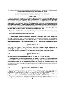
which have been regarded fast for solving (8). All experiments were performed under Windows Vista Premium and MATLAB v7.6 (R2008a) running on a Lenovo laptop with an Intel Core 2 Duo CPU at 1.8 GHz and 2 GB of memory. We generated our test sets using three images, the SheppLogan phantom image and two brain MR images, with different sampling ratios. In each test, we generated the data fp in (7) by first rescaling the intensity values of the tested image to [0, 1] followed by applying a partial FFT and adding Gaussian noise. To apply a partial FFT, we sampled the Fourier domain along a number of radial lines (RLs) spread out from the center; for example, Figure 1 shows 22 radial lines in a Fourier domain.

Fig. 1.

Fourier domain sampling positions with 22 radial lines for test 1.

In all tests, the additive Gaussian noise had a mean zero and standard deviation 0.01. We tried different starting points for the three algorithms and found that all of them are insensitive towards starting points. Therefore, we simply initialized the starting image u by zero. Table I summarizes the test data, as well as the values of the parameters λ and τ used in (8). TABLE I T EST IMAGES INFORMATION AND MODEL PARAMETER VALUES Test 1 2 3

Image phantom brain-1 brain-2

Size 256 × 256 256 × 256 512 × 512

RLs 22 44 44

Sample Ratio 9.36% 18.76% 9.64%

(λ, τ ) (1e2∼1e5, 0) (2e3, 1) (2e3, 1)

It is important to note that both TwIST and OS can be applied to problem (8) with Fp being replaced by a general linear operator A as long as Au and A> u are computable, but RecPF is limited to the cases where T in (7) must correspond to an orthogonal matrix that can diagonalize the finite difference operators D(1) and D(2) under suitable boundary conditions (e.g., T can be a FFT (or DCT) matrix together with the periodic (or symmetric) boundary conditions imposed on u). In addition, both TwIST and OS solve a scaled version of (8) where the objective function in (8) is scaled by 1/λ. To keep compatibility, we multiply the objective function by 1/λ for RecPF. Hence, the objective values presented below for (λ, τ ) were scaled by 1/λ. B. Comparison with TwIST In test 1, we compare RecPF with TwIST, which in general solves 1 min λ−1 Φreg (u) + kAu − bk2 , u 2

where Φreg (·) can be either TV or `1 regularization and A is a linear operator. The iteration framework of TwIST is uk+1 = (1 − α)uk−1 + (α − δ)uk + δΨλ (ξk ), where α, δ > 0 are parameters, ξk = uk + A> (b − Auk ), and Ψλ (ξk ) = arg min λ−1 Φreg (u) + (1/2) · ku − ξk k2 . u

(30)

Its latest version, TwIST v1, cannot solve problem (8) with both the TV and `1 regularization terms. Hence, in order to compare RecPF with TwIST on the same model, we drop the `1 -term P in (8) by setting τ = 0 for RecPF and letting Φreg = i kDi uk2 and A = Fp for TwIST. In TwIST v1, the subproblem (30) is solved iteratively by Chambolle’s algorithm [9]. In comparison, RecPF with the `1 term dropped has a per-iteration cost of 3 FFTs (including 1 inverse FFT), which is much lower than solving (30) by Chambolle’s algorithm. This is one of the main reasons that RecPF runs faster. We set the stopping parameter ² = 10−3 in (20) for RecPF, and used the monotonic variant of TwIST in TwIST v1, which was stopped when the relative change in the objective function falled below tol = 10−3 . In TwIST v1, the parameters α and δ are determined carefully based on the spectral distribution of A> A. Under the circumstance, the minimum and maximum eigenvalues of A> A are obviously 0 and 1, respectively. Therefore, we assigned a relatively small value 10−3 to the TwIST parameter lam1 (which determines α and δ), as recommended by the TwIST v1 documentation. Table II gives the performance results of RecPF and TwIST for different values of λ. We also tested TwIST with lam1= 10−4 , but do not include the obtained results since they are similar to those for lam1= 10−3 . Table II lists the following quantities: the error in the reconstructed image relative to the original image (Err), the final objective function value (Obj), the number of iterations (Iter), and the CPU time in seconds (CPU). TABLE II R ESULTS ON T EST 1. λ 1e+2 1e+3 1e+4 1e+5

Err 5.4% 4.4% 43.4% 43.5%

TwIST Obj Iter 15.15 25 1.919 106 .4452 10 .1368 10

CPU 25 66 11 9

Err 8.6% 4.5% 4.8% 4.9%

RecPF Obj Iter 14.79 180 1.838 195 .2998 187 .1359 186

CPU 15 16 15 15

We point out that upon termination RecPF returned smaller objective values than TwIST for both λ = 102 and λ = 103 , though the solutions from TwIST have slightly smaller relative errors. For λ = 104 , TwIST failed to converge with tol = 10−3 and obtained an image with relative error 43.4%. In this case, if tol is decreased from 10−3 to 10−4 without other changes, TwIST obtained a solution with relative error 7.1% but in much longer CPU time (about 280 seconds). For λ = 105 , similar phenomena happened except TwIST also failed with tol = 10−4 . From Table II, it can be seen that RecPF is faster than TwIST to attain a comparable accuracy. This is primarily because of the difference in per-iteration costs of the two: TwIST solves the TV problem (30) using Chambolle’s algorithm (that

7

requires its own iteration loop), while RecPF solves (16) at an approximate cost of 3 FFTs. In terms of the iteration numbers and CPU time consumed, RecPF is relatively stable as λ varies while TwIST appears to be sensitive. The reconstructed images corresponding to λ = 103 appear to have the best quality, and are given in Figure 2.

corresponding to the positions where samples have been taken; and (ii) as λ gets larger, the entries of F(u) corresponding to the sampled positions gets closer to fp . In the limit as λ → ∞, solving (17) simply fills F(u) with fp at the sampled positions, and updates the remaining entries of F(u) independent of λ. This separation makes RecPF very stable with large λ and allows it to faithfully retain the effect of TV regularization. C. Comparison with OS In tests 2 and 3, we compare RecPF with OS [17] on solving problem (8) with both TV and `1 terms. OS iterates the fixpoint equations (31) below, in which s ∈ RN , wi , ti ∈ R2 , i = 1, . . . , N , are auxiliary variables and δ1 , δ2 > 0 are constants:  ¡P > ¢ s = Ψ> u − (δ1 /λ) · Ψ>  i Di wi + λ∇θ(u, fp ) ,   t = w + δ D u, ∀i, i i 2 i (31)  u = Ψ {max (|s| − δ1 τ /λ, 0) ◦ sgn(s)} ,    wi = min (1/δ2 , kti k) · ti /kti k, ∀i.

Fig. 2. Reconstructed images in test 1. Top left: original image. Top right: reconstruction by TwIST with λ=1e+3 (Err = 4.42%). Bottom left: reconstruction by RecPF with λ=1e+3 (Err = 4.48%). Bottom right: reconstructed by RecPF with λ=1e+10 (Err = 4.89%).

We also tested the two algorithms on data containing less or no noise and observed similar relative performances. For example, on noiseless data, both algorithms were able to converge to solutions with relative errors less than 1% for λ = 103 , but RecPF was faster than TwIST. In these experiments, we found that TwIST v1 seems to require careful selections of parameters such as α, δ, λ and error tolerance tol in order to obtain results comparable to those of RecPF. This behavior is exemplified by the fact that TwIST failed for (λ, tol) = (104 , 10−3 ) or (105 , 10−4 ) by returning solutions with relative errors over 40% (similar behavior happened for lam1= 10−4 as well), while it did return a good solution with (λ, tol) = (104 , 10−4 ) at a cost of more iterations and a longer CPU time. We tested different stopping criteria provided by TwIST v1 and found that the above cases apparently were not isolated cases. In comparison, RecPF is simple and requires little tuning. As mentioned, the default setting given in Algorithm 2 was used throughout our tests where only the error tolerance ² in (20) was varied. Interestingly, the performance of RecPF appears to be totally insensitive to the values of λ, and it converges well even with huge λ values. For example, we tested RecPF with λ = 1010 and obtained an image with relative error 4.89%, which is depicted at the bottom right corner in Figure 2. We tested even larger λ and obtained equally good images. This behavior can be explained by closely examining the linear system in (17). Recall that η = λ/β and P is a selection matrix. From the ˆ and rˆ below (17) it becomes clear that (i) formulations of L the value of λ only affects those Fourier coefficients in F(u)

The authors showed that for any fixed δ1 , δ2 > 0, u is a solution of (8) if and only if it satisfies (31). Given uk and {wik , ∀i}, sk and {tki , ∀i} can be computed by the first two equations, and then be used to compute uk+1 and {wik+1 , ∀i} in the last two equations in (31). For δ1 and δ2 in certain range, such iterations converge. Similar to RecPF, every iteration of OS involves shrinkages, FFTs and discrete wavelet transforms (DWTs), and OS also has continuation, decreasing τ and 1/λ from larger values to prescribed small ones. For a fixed pair of (τ, λ), the fixed-point iterations of OS terminate if one of the following two conditions are met: p fk − fk+1 < ε2 τc /τt max{1, fk }, (32) kuk+1 − uk k < ε1 max{1, kuk k},

(33)

where fk is the objective value at uk , τc and τt are the current and the target values of τ , respectively, and ε1 , ε2 > 0 are stopping tolerances. In both tests, we set δ1 = δ2 = 0.8, ε1 = 10−4 and ε2 = 5 × 10−4 for OS. For RecPF, we set the stopping tolerance ² = 2.5 × 10−2 in (20) which, although much looser than the previous tolerance used in test 1, is sufficient to obtain better results than OS. Since the two algorithms use different stopping criteria and OS has multiple tuning parameters such as δ1 and δ2 that influence the convergence speed, it is rather difficult to compare them at their best performance. Since OS implements the fixed-point iterations based on (31) that do not directly aim at decreasing the objective function, its objective values do not decrease monotonically for certain choices of δ. We tried different δ values and observed the following. For smaller δ’s, OS tends to yield monotonically decreasing objectives but converges slowly. For larger δ’s and looser stopping criteria, OS becomes faster but loses objective monotonicity and returns solutions with larger relative errors. After having tried different combinations of ε’s and δ’s for OS, we determined to use the above parameter values in the results presented below as a best compromise between convergence speed and image quality.

8

In both tests 2 and 3, the sparsity promoting basis Ψ was set to be the Haar wavelet transform using the Rice Wavelet Toolbox in its default setting [18]. The per-iteration computational cost of RecPF is 4 FFTs (including 1 inverse FFT) and 2 DWTs (including 1 inverse DWT). It is not difficult to check from (31) that the per-iteration cost of OS is 2 FFTs less than that of RecPF. Considering this difference, we present our numerical results in plots of objective value and relative error versus CPU time in Figures 3 and 4, respectively. The reconstructed images are give in Figure 5. Test 2−RecPF Test 2−OS Test 3−RecPF Test 3−OS

Objective function

3

10

2

Our other experiments yielded consistent results. In general, when stricter tolerances are used, better results can be obtained from both algorithms at a cost of longer CPU times. Independent of tolerances used, their performance difference stay with a similar ratio.

10

1

10

0

Fig. 3.

5

10

15

CPU time (sec)

V. C ONCLUSION

Comparing RecPF with OS: objective value versus CPU time.

Based on the classic penalty function approach in optimization, a highly efficient alternating minimization algorithm, called RecPF, was proposed for reconstructing large-scale signals or images from a subset of their frequency data (DFT or DCT coefficients). The algorithm minimizes a potential function with one or both of TV and `1 -norm regularization terms. At each iteration, the main computation of RecPF only involves fast and stable operations consisting of shrinkages and FFTs (or DCTs). RecPF enjoys strong convergence properties and its practical convergence is accelerated by continuation on penalty parameters. RecPF is compared to two efficient algorithms TwIST [3] and OS [17], which can solve problems with broader data types than RecPF. On image reconstruction problems with frequency data, the strong numerical evidence presented in this paper shows that RecPF is able to take the advantage of the frequency date type and achieves much higher performance in terms of both reconstruction speed and quality than TwIST and OS. It is hoped that RecPF can be useful in relevant areas of compressive sensing such as sparsity-based, rapid MR image reconstruction.

1 Test 2−RecPF Test 2−OS Test 3−RecPF Test 3−OS

0.9 0.8

Relative error

0.7 0.6 0.5 0.4 0.3 0.2 0.1 0

0

2

4

6

8

10

12

14

CPU time (sec). Fig. 4.

Fig. 5. Results of tests 2 (top row, 256×256) and 3 (bottom row, 512×512). Left column: original brain images. Middle column: reconstructed by OS, Err: 15.02% (upper) and 14.73% (lower). Right column: reconstructed by RecPF, Err: 10.97% (upper) and 11.58% (lower).

Comparing RecPF with OS: relative error versus CPU time.

As can be seen from Figures 3 and 4, both algorithms converged faster in test 2 where relatively more data were collected, and RecPF converged faster than OS in terms of both objective functions and relative errors. Moreover, images reconstructed by RecPF have higher qualities than those by OS as is evidenced by Figure 5. In addition, in both tests RecPF achieved and maintained both lower objective values and relative errors throughout the entire iteration process. This is most evident in test 3, in which RecPF took much less CPU time than OS to attain the same level of relative error.

A PPENDIX A P ROOF OF T HEOREM 3.4 From (13), for any i ∈ {1, . . . , N }, it holds that kwik+1 − wi∗ k2

° °2 = °s2 ◦ gi (v k ) − s2 ◦ gi (v ∗ )° ° °2 ≤ °gi (v k ) − gi (v ∗ )° . (34)

9

Suppose wik+1 6= 0 for some i ∈ L2 , then

and

kwik+1 − wi∗ k2 ° °2 = °s2 ◦ gi (v k ) − s2 ◦ gi (v ∗ )° ¡ ¢2 = kgi (v k )k − 1/β © ª2 ≤ kgi (v k ) − gi (v ∗ )k − (1/β − kgi (v ∗ )k) 2

≤ kgi (v k ) − gi (v ∗ )k2 − (1/β − kgi (v ∗ )k) ≤ kgi (v k ) − gi (v ∗ )k2 − ω22 ,

(35)

where the first equality comes from the iteration of wi in (13) and the definition of gi (v); the second equality holds because of kgi (v ∗ )k < 1/β, wik+1 6= 0 and the definition of s2 ; the first inequality is triangular inequality; the second inequality follows from the fact that kgi (v k )−gi (v ∗ )k ≥ 1/β− kgi (v ∗ )k > 0; and the last one uses the definition of ω2 in (29). Furthermore, kz

k+1

∗ 2

−z k

(1)

k

(1)

= kS1 ◦ h (v ) − S1 ◦ h ≤ kh(1) (v k ) − h(1) (v ∗ )k2 .

∗

(v )k

2

(36)

Combining (34), (35) and (36), we get kv k+1 − v ∗ k2

= kz k+1 − z ∗ k2 + kwk+1 − w∗ k2 X = kz k+1 − z ∗ k2 + kwik+1 − wi∗ k2 (1)

k

(1)

≤ kh (v ) − h (v )k2 X + kgi (v k ) − gi (v ∗ )k2 − ω22

(37)

Therefore, for i ∈ L2 , it holds that wik = wi∗ = 0 in no more than kv 0 − v ∗ k2 /ω22 iterations. Similarly, for any i ∈ {1, . . . , N }, from (11) we have ´2 ³ ¡ k+1 ¢2 (1) (1) zi − zi∗ = s1 ◦ hi (v k ) − s1 ◦ hi (v ∗ ) ¯ ¯2 ¯ (1) ¯ (1) ≤ ¯hi (v k ) − hi (v ∗ )¯ . (38) Suppose zik+1 6= 0 for some i ∈ L1 , similar discussion as in (35) gives ¯2 ¡ k+1 ¢2 ¯¯ (1) ¯ (1) zi − zi∗ ≤ ¯hi (v k ) − hi (v ∗ )¯ − ω12 , (39) where ω1 is defined in (28). Combining (34), (38) and (39), similar arguments as in (37) gives (40)

Therefore, zik = zi∗ = 0 in no more than kv 0 − v ∗ k2 /ω12 iterations for i ∈ L1 . A PPENDIX B P ROOF OF T HEOREM 3.5 From (24)–(27), there hold uk+1 − u∗ = M −1 H > (v k+1 − v ∗ )

kv k+1 − v ∗ k2 ≤ kHM −1 H > (v k − v ∗ )k2 = kT (v k − v ∗ )k2 . Since we are only interested in the asymptotic behavior of k Algorithm 1, without loss of generality, we assume that vL = ∗ vL = 0. The above inequality becomes k+1 ∗ 2 kvE − vE k

k ∗ > k ∗ ≤ (vE − vE ) (T 2 )EE (vE − vE ) 2 k ∗ 2 ≤ ρ((T )EE )kvE − vE k ,

which implies assertion 1 of this theorem. Multiplying H on k both sides of (41), from vL = 0 and (42), we get kH(uk+1 − u∗ )k2

k+1 k+1 ∗ > ∗ ≤ (vE − vE ) (T 2 )EE (vE − vE ) ≤ ρ((T 2 )EE )kH(uk − u∗ )k2 ,

ACKNOWLEDGMENT

i

kv k+1 − v ∗ k2 ≤ kv k − v ∗ k2 − ω12 .

Combining the recursion (41), (42) and the definition of T , it holds

which completes the proof of Theorem 3.5.

i ∗

= kh(v k ) − h(v ∗ )k2 − ω22 ≤ kv k − v ∗ k2 − ω22 .

= = + ≤ =

kv k+1 − v ∗ k2 kz k+1 − z ∗ k2 + kwk+1 − w∗ k2 kS1 (Ψ> uk ) − S1 (Ψ> u∗ )k2 kS2 (D(1) uk ; D(2) uk ) − S2 (D(1) u∗ ; D(2) u∗ )k2 kΨ> (uk − u∗ )k2 + kD(uk − u∗ )k2 kH(uk − u∗ )k2 . (42)

(41)

The work of J. Yang has been supported by the Chinese Scholarship Council during his visit to Rice University. The work of Y. Zhang has been supported in part by NSF Grant DMS-0811188 and ONR Grant N00014-08-1-1101. The work of W. Yin has been supported in part by NSF CAREER Award DMS-0748839 and ONR Grant N00014-08-1-1101. R EFERENCES [1] R. Baraniuk, M. Davenport, R. DeVore, and Michael Wakin, A simple proof of the restricted isometry property for random matrices, Constructive Approximation, to appear. [2] D. Baron, M. Duarte, S. Sarvotham, M. B. Wakin, and R. G. Baraniuk, Distributed compressed sensing, Available at: http://dsp.rice.edu/cs/DCS112005.pdf. [3] J. Bioucas-Dias, and M. Figueiredo, A new TwIST: Two-step iterative thresholding algorithm for image restoration, IEEE Trans. Imag. Process., vol. 16, no. 12, pp. 2992–3004, 2007. [4] E. Cand` es, and J. Romberg, Practical signal recovery from random projections, http://www.dsp.ece.rice.edu/cs, Compressed Sensing Resources. [5] E. Cand` es, J. Romberg, and T. Tao, Stable signal recovery from incomplete and inaccurate information, Communications on Pure and Applied Mathematics, vol. 59, pp. 1207-1233, 2005. [6] E. Cand` es, J. Romberg, and T. Tao, Robust uncertainty principles: Exact signal reconstruction from highly incomplete frequency information, IEEE Trans. Inform. Theory, vol. 52, no. 2, pp. 489–509, 2006. [7] E. Cand` es, and T. Tao, Decoding by linear programming, IEEE Trans. Inform. Theory, vol. 51, no. 12, pp. 4203–4215, 2005. [8] E. Cand` es, and T. Tao, Near optimal signal recovery from random projections: Universal encoding strategies, IEEE Trans. on Inform. Theory, vol. 52, no. 12, pp. 5406 – 5425, 2006. [9] A. Chambolle, An algorithm for total variation minimization and applications, J. Math. Imaging Vision., 20, pp. 89–97, 2004. [10] S. S. Chen, D. L. Donoho, and M. A. Saunders, Atomic decomposition by basis pursuit, SIAM J. Scientific Computing vol. 20, 33–61, 1998. [11] R. Courant, Variational methods for the solution of problems with equilibrium and vibration, Bull. Amer. Math. Soc., 49, pp. 1–23, 1943.

10

[12] D. Donoho, Compressed sensing, IEEE Trans. Inform. Theory, vol. 52, no. 4, pp. 1289–1306, 2006. [13] D. Donoho, For Most Large Underdetermined Systems of Linear Equations, the minimal l1-norm solution is also the sparsest solution, Communications on pure and applied mathematics, Vol. 59, No. 7, pp. 907–934, 2006. [14] D. Geman and C. Yang, Nonlinear image recovery with half-quadratic regularization, IEEE Trans. Image Process., vol. 4, pp. 932–946, 1995. [15] L. He, T.-C. Chang, S. Osher, T. Fang, and P. Speier, MR image reconstruction by using the iterative refinement method and nonlinear inverse scale space methods, UCLA CAM Report 06-35, 2006. [16] M. Lustig, D. Donoho, and J. Pauly, Sparse MRI: The application of compressed sensing for rapid MR imaging, Magnetic Resonance in Medicine, vol. 58, no. 6, pp. 1182–1195, 2007. [17] S. M A , W. Y IN , Y. Z HANG , AND A. C HAKRABORTY, An efficient algorithm for compressed MR imaging using total variation and wavelets, IEEE Conference on CVPR, pp. 1–8, 2008. [18] Rice Wavelet Toolbox, http://www.dsp.rice.edu/software/rwt.shtml. [19] J. A. Tropp, and A. C. Gilbert, Signal recovery from random measurements via orthogonal matching pursuit, IEEE Trans. Inform. Theory, vol. 53, no. 12: 4655-4666, 2007. [20] Y. Wang, J. Yang, W. Yin and Y. Zhang, A new alternating minimization algorithm for total variation image reconstruction, SIAM J. Imag. Sci., vol. 1, no. 4, 248–272, 2008. [21] J. Yang, W. Yin, Y. Zhang, and Y. Wang, A fast algorithm for edgepreserving variational multichannel image restoration, TR08-09, CAAM, Rice University, Submitted to SIIMS. [22] J. Yang, Y. Zhang, and W. Yin, An efficient TVL1 algorithm for deblurring of multichannel images corrupted by impulsive noise, TR0812, CAAM, Rice University, Submitted to SISC. [23] Y. Zhang, On theory of compressive sensing via `1 -minimization: simple derivations and extensions, TR08-11, CAAM, Rice University. Submitted to SIREV.