A Fast Multilevel Algorithm for Wavelet-Regularized Image Restoration

IEEE TRANSACTIONS ON IMAGE PROCESSING, VOL. 18, NO. 3, MARCH 2009

509

A Fast Multilevel Algorithm for Wavelet-Regularized Image Restoration Cédric Vonesch and Michael Unser, Fellow, IEEE

Abstract—We present a multilevel extension of the popular “thresholded Landweber” algorithm for wavelet-regularized image restoration that yields an order of magnitude speed improvement over the standard fixed-scale implementation. The method is generic and targeted towards large-scale linear inverse problems, such as 3-D deconvolution microscopy. The algorithm is derived within the framework of bound optimization. The key idea is to successively update the coefficients in the various wavelet channels using fixed, subband-adapted iteration parameters (step sizes and threshold levels). The optimization problem is solved efficiently via a proper chaining of basic iteration modules. The higher level description of the algorithm is similar to that of a multigrid solver for PDEs, but there is one fundamental difference: the latter iterates though a sequence of multiresolution versions of the original problem, while, in our case, we cycle through the wavelet subspaces corresponding to the difference between successive approximations. This strategy is motivated by the special structure of the problem and the preconditioning properties of the wavelet representation. We establish that the solution of the restoration problem corresponds to a fixed point of our multilevel optimizer. We also provide experimental evidence that the improvement in convergence rate is essentially determined by the (unconstrained) linear part of the algorithm, irrespective of the type of wavelet. Finally, we illustrate the technique with some image deconvolution examples, including some real 3-D fluorescence microscopy data. Index Terms—Bound optimization, confocal, convergence acceleration, deconvolution, fast, fluorescence, inverse problems, -regularization, majorize-minimize, microscopy, multigrid, multilevel, multiresolution, multiscale, nonlinear, optimization transfer, preconditioning, reconstruction, restoration, sparsity, surrogate optimization, 3-D, variational, wavelets, widefield.

I. INTRODUCTION A. Motivation and Originality of the Present Work

I

NVERSE problems arise in various imaging applications such as biomicroscopy [1], [2], medical imaging [3], [4], or astronomy [5], [6]. An increasingly important issue for reconstruction and restoration tasks is the mass of data that is now routinely produced in these fields. The instrumentation typically Manuscript received March 10, 2008; revised September 29, 2008. First published February 2, 2009; current version published February 11, 2009. This work was supported in part by the Hasler Foundation. The associate editor coordinating the review of this manuscript and approving it for publication was Dr. Pier Luigi Dragotti. The authors are with the Biomedical Imaging Group, EPFL, Lausanne, Switzerland (e-mail: [email protected]; [email protected]). Color versions of one or more of the figures in this paper are available online at http://ieeexplore.ieee.org. Digital Object Identifier 10.1109/TIP.2008.2008073

allows for high-dimensional and multimodal imaging, fostering the evolution of experimental practices towards more quantitative and systematic investigations. This trend will arguably persist over the forthcoming years, and, as a result, computation time will remain a serious bottleneck for restoration methods, despite the progress of computer hardware. In this context, advanced (nonlinear) restoration methods that were developed for traditional 2-D imaging cannot be applied directly; larger-scale problems require more efficient algorithmic implementations. The concept of “sparsity” has drawn considerable interest recently, leading to a new and successful paradigm for the regularization of inverse problems. The main idea is to constrain the restored image to have only a few nonzero coefficients in a suitable transform domain. Based on this principle, a simple and elegant iterative algorithm—which we shall call the “thresholded Landweber” (TL) algorithm—was independently derived by several research groups [7]–[9]. The method has the advantage of being very general. However, it is known to converge slowly when applied to ill-conditioned inverse problems [10]–[12], which restrains its suitability for large data sets. In this paper, we construct a multilevel version of the TL algorithm that is significantly faster; this allows us to apply the method for the restoration of real 3-D multichannel fluorescence micrographs. To do so, we specifically consider the case where the sparsity constraint is enforced in the wavelet domain, which was shown to yield state-of-the-art results for 2-D image restoration (see [7]). From a numerical standpoint, the advantage of using wavelet representations is twofold. First, their tree structure naturally leads to efficient computational schemes in the spirit of Mallat’s Fast Wavelet Transform [13]. Second, the spectral localization properties of wavelets make them suitable for preconditioning, that is, for partly compensating the poor conditioning of the inverse problem. The structure and the convergence speed of our multilevel algorithm make it comparable to multigrid schemes [14], [15]. These schemes belong to the most efficient known methods for the numerical resolution of partial differential equations; they are typically one order of magnitude faster than standard iterative methods. In fact, the connection between wavelet and multigrid theory was recognized early on [16]–[19]. Surprisingly, though, the potential of wavelet-based multilevel methods for image restoration has hardly been exploited so far. An exception is the paper by Wang et al. [20], which is, however, restricted to linear restoration and based on a relatively empirical reformulation of the image-formation model in the wavelet domain. Our approach is based on a nonquadratic variational formulation (leading to a nonlinear restoration method) and on the principle of bound optimization [21], [22]. This principle also

1057-7149/$25.00 © 2009 IEEE Authorized licensed use limited to: EPFL LAUSANNE. Downloaded on February 24, 2009 at 05:34 from IEEE Xplore. Restrictions apply.

510


underlies the derivation of [8] and is known under several alternative denominations, such as optimization transfer, surrogate functional optimization or majorize-minimize (MM) strategy. Our method can be related to the family of “block-alternating MM algorithms” [23]. In the context of statistical signal processing, one of the earliest representatives of this family is the “Space-Alternating Generalized EM” (SAGE) algorithm of Fessler and Hero [24]. More recently, a bound-optimization approach was also used by Oh et al. to derive a multigrid inversion method for nonlinear problems [25]. While the works [23]–[25] do not involve wavelets, the latter can be related to the so-called lazy wavelet transform [26], which itself corresponds to the anterior concept of hierarchical basis in the finite element and multigrid literature [27], [28]. Similarly, our work can be related to generalizations of the hierarchical-basis method [17], [29]. To achieve our goal, we construct a family of bounds that allow us to divide the original variational problem into a collection of smaller problems, corresponding to the different scales of the wavelet decomposition. The bounds can be made particularly tight for specific subbands. This leads to subband-dependent iteration parameters (step sizes and threshold levels), which are the key to faster convergence. The bound optimization framework provides a rationale for choosing these parameters in a consistent manner. At the same time, this framework is simple to deploy and guarantees that the underlying cost functional is monotonically decreased. B. Image-Formation Model We will be concerned with the recovery of signals that are distorted by a linear measurement device and noise. Throughout the paper, we will use a discrete description where the measured signal is given by the algebraic relation

Here, the vector holds lexicographically ordered samples of the original -dimensional signal ( is the product of the number of samples along each is a transform matrix modeling the image-fordimension). mation device and represents the noise component. from the measureThe estimation of the original signal ment is an ill-posed inverse problem [30]. Most approaches for overcoming this ill-posedness can be described in a variational framework, where one looks for an estimate that minimizes a predefined cost functional. This functional is typically the sum of a data term and a regularization term. Without going into the details of a Bayesian interpretation [5], [7], the former term enforces a certain level of consistency between the estimate and the measured signal (with respect to the image-formation model). The latter term prevents overfitting—and, thus, instability—by favoring estimates that are close to some desirable class of solutions (according to some regularity measure). C. Regularized Inversion Using a Wavelet-Domain Sparsity Constraint The discovery that natural images can be well approximated using only a few large wavelet coefficients can be traced back to the seminal work of Mallat [13] and is, for example, exploited

in the JPEG2000 compression format [31]. Following several recent works (see below), we will use a regularization term that promotes estimates with a sparse wavelet expansion; the data term will be a standard quadratic criterion. In the sequel, we assume that the reader is familiar with the filter-bank implementation of the wavelet transform [26]. We will denote by the vector that contains the coefficients of an estimate in a preassigned wavelet basis; we shall refer to this basis as the synthesis wavelet basis. Introducing the synthesis , whose columns are the elements of this basis, we matrix can write that

Later in this paper, we will also use the analysis matrix , whose columns are the elements of the dual wavelet basis. The perfect-reconstruction condition can be expressed as , where denotes transposition (or Hermitian transposition in the case of a complex wavelet transform). Note that the present formulation also includes the case of overcomplete wavelet repare then nonsquare matrices). resentations ( and With these notations, we consider that a solution to the in, where minimizes the verse problem is given by functional (1) Here, represents the -norm of the wavelet coefficients, that is, the sum of their absolute values. Compared to the stan), the -norm puts more dard Euclidian norm (denoted by weight on small coefficients, and less weight on large coefficients. Thus, depending on the magnitude of the regularization parameter , it favors estimates whose energy is mostly concentrated in a few large wavelet coefficients. Note that in general the coarsest-scale scaling-function coefficients are not included in the regularization term (see Section III-C for more details). An algorithm for the minimization of (1) has been derived in [7]–[9], as well as in the earlier works [32], [33]. A similar procedure is also described in [34], [35]. The beauty of the method resides in its simplicity: it essentially consists in alternating between a Landweber iteration [36] and a waveletdomain thresholding operation [37]—hence the name “thresholded Landweber” (TL) algorithm. When is adequately noris orthonormal (implying that ), malized and the TL algorithm can be described by the recursive update rule1 (2) starting from some arbitrary initial estimate . Here, stands for a pointwise application of the well-known soft-threshas olding function [38], which can be defined for

where

if otherwise.

1To keep the notations simple, we do not introduce a specific index to distinguish between the individual estimates. Instead, we use the assignment operator “ ” whenever a quantity (such as the estimate) is updated. The algorithmic signification of this operator is that the expression on the right-hand side is evaluated and the result is stored in the left-hand side variable

Authorized licensed use limited to: EPFL LAUSANNE. Downloaded on February 24, 2009 at 05:34 from IEEE Xplore. Restrictions apply.

VONESCH AND UNSER: FAST MULTILEVEL ALGORITHM FOR WAVELET-REGULARIZED IMAGE RESTORATION

The presence of in (2) guarantees that a certain fraction of wavelet coefficients will be set to zero, depending on the magnitude of the regularization parameter . D. Recent Relevant Work and Objectives of the Paper The present work represents a substantial extension of a previous algorithm of ours [12], which was specific to convolutive image-formation operators and to a sparsity constraint in the (bandlimited) Shannon wavelet basis [26]. Here, the goal is to derive a comparably fast algorithm for an arbitrary wavelet basis, without making the assumption that the image-formation operator leaves the different subbands uncoupled. The approach described in the present paper differs fundamentally from [12] in that it is based on a sequential update of the wavelet subbands, instead of a parallel update. This requires a more sophisticated multilevel algorithm. Similarly to what is done in some presentations of the multigrid methodology—where a “model problem” is often used to convey the intuition [15]—we will motivate and illustrate our approach in the context of deconvolution. In this case, can be thought of as a (block-)circulant matrix corresponding to a given convolution kernel; our multilevel method is then particularly efficient, thanks to the shift-invariant structure of the wavelet subspaces. However, its principle can be applied to more general inverse problems. The most direct extension can be approxconcerns inverse problems for which imated by a convolution matrix—specifically tomographic corresponds to a discretized image-reconstruction, where Radon transform. The subclass of inverse problems involving a )—e.g., unitary image-formation operator (such that denoising, reconstruction from K-space (frequency-domain) samples or digital holography microscopy [39]—may also benefit from the method. In the present work, we have tried to provide a general and modular pseudo-code description of the multilevel TL algorithm that is readily transposable to machine implementation. Several works have already extended the standard TL algorithm (which was originally formulated only for orthonormal bases) to more general decompositions, including overcomplete wavelet representations [10], [40]. Nevertheless, the principle and the convergence properties of the algorithm were not fundamentally changed in these settings (although [40] is based on a quite different proximal thresholding interpretation). Faster methods for the minimization of (1) have only been proposed very recently. We are aware of two-step methods [11], [41], [42], line-search methods [43]–[45], coordinate-descent methods ([46] and also [43] and [44]) and a domain-decomposition method [47]. The latter is based on a well-established concept from the finite-element literature, so that it is arguably the closest to our approach. However, it is not specific to wavelets and relies entirely on dimension-reduction effects for decreasing the computational complexity. The above methods differ with respect to the number and the determination of their step sizes. Among the fixed-step-size strategies, the domain-decomposition approach [47] uses the same step size for all subspaces, whereas the coordinate-descent methods described in [43], [44], and [46] use step sizes that are adapted to each atom individually. The methods of Bi-

511

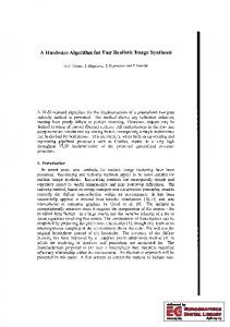
oucas-Dias, Figueiredo, and Nowak [11], [41], [42] have the advantage of simplicity, because they use only two iteration parameters that are also determined a priori (however, these parameters may require some hand tuning based on the outcome of a small number of preliminary iterations). The principle of the line-search methods [43]–[45] is that the step sizes are adjusted depending on the context, which involves additional computations at every iteration. Our algorithm is somewhere in between all these approaches: the step sizes are adjusted at the level of individual wavelet subbands, they can be precomputed for a given image-formation operator and wavelet family, and they remain fixed during the entire algorithm. In summary, to the best of our knowledge, a wavelet-based multilevel method comparable to ours—which combines cyclic updates of the different resolution levels with the preconditioning effect of subband-specific iteration parameters—has not been proposed so far. Therefore, we have chosen to focus on the derivation and the experimental validation of our algorithm. A theoretical study of its convergence properties and a comparison with the aforementioned techniques is a research subject in its own right that will certainly be investigated in the future. The remainder of the paper is organized as follows. In Section II, we revisit the derivation of the TL algorithm (2) which was presented in [8], introducing additional degrees of freedom into the bound optimization framework. This leads to our multilevel algorithm, described in Section III. Section IV is dedicated to numerical experiments. II. DIVIDE—THE THRESHOLDED LANDWEBER ALGORITHM, REVISITED A. Notations In this section, we will primarily be interested in the subspace structure of the wavelet representation. The tree-structure of the wavelet transform—that is, the embedding of the underlying scaling-function subspaces—will become important for the algorithmic considerations of the next section. To account for both aspects, we introduce the following notations, which are illustrated in Fig. 1. Throughout this paper, we shall use the terms “scale,” “resolution level,” “decomposition level,” and “level” interchangeably. • : number of resolution levels of the wavelet representation ( : scale index). : number of wavelet subbands at scale , excluding the • scaling-function subband ( : subband index). : general subband index. Our convention will be • that corresponds to the scaling-function subband at scale ; however, for the sake of conciseness, we will often . The context will indicate simply write instead of whether we are referring to the scaling-function subband or to the decomposition level. : indexing set for • . At the all wavelet subbands at a scale coarsest level, we include the scaling-function subband: . • : indexing set for all subbands produced by a -scale decomposition (including the coarsest-scale scaling-function subband)


512


Fig. 1. Complementary notations reflecting the tree structure (notations associated with continuous lines) and the subspace structure (notations associated with . The number of subbands is at every scale , which is dashed lines) of the wavelet representation. Here, the number of decomposition levels is typical for a 2-D separable wavelet representation.

, the idea is to iteratively construct original cost functional a series of auxiliary functionals that are easy to minimize. , say , we Given an estimate of the minimizer of define •

: wavelet or scaling-function coefficients of the current estimate corresponding to subband . is the concatenafor every . Note that is an alias for . tion of : matrix corresponding to the reconstruction part (up• sampling and filtering using the synthesis filters) of the channel of the filter bank at scale , to go from to . : “restriction” of the synthesis matrix to subband , • such that (3) More precisely, this is a cascade of upsampling and filtering operations defined recursively by for

.

(4)

(6) This functional has three important characteristics. , takes the same value as . 1) When is an upper-bound of , 2) For all other values of , by virtue of (5). 3) admits a minimizer with a closed-form expression. The first two properties imply that, if we find a new estimate that minimizes (or at least decreases) , we also decrease . We simply have to observe that

The third property allows us to actually construct such a new estimate. It originates from the negative (rightmost) term in (6), which cancels out the coupling of the wavelet coefficients in . As a result, the auxiliary functional can be rewritten as

B. Estimation of the Cost Functional Using Subband-Dependent Bounds

(7)

Our algorithm is based on the availability of a wavelet-domain estimation of that takes the following form: we assume such that that there are constants (5) We shall assume for now that this inequality holds for an arbitrary vector of wavelet coefficients , and we shall revisit the derivation of the bound-optimization algorithm of Daubechies et al. [8]. Rather than directly considering the

where the constant does not depend on . This expression reveals that the auxiliary functional is essentially a weighted sum of “subfunctionals” that depend on distinct subbands. Furthermore, the wavelet coefficients appear to be completely decoupled in each subfunctional. This means that once we have comfor every subband , we puted can minimize each subfunctional using solely pointwise operations. This minimization procedure can be related to two standard image-restoration methods. First, the computation of



may be seen as a wavelet-domain Landweber iteration [30], [36]: the wavelet decomposition of the “reblurred residual” serves as a correction-term, which is applied with a (subband-dependent) step size . Let us point out, however, that the decomposition of the residual must be performed using the synthesis basis. Second, each subfunctional can be interpreted as a denoising functional where represents the wavelet coefficients of a signal to be denoised and is a regularization parameter (again subband-dependent). The minimizer of such a functional is unique and is obtained by soft-thresholding the coefficients of the noisy signal, with a threshold level equal to half the regularization parameter [48]. C. Relation With the Standard Thresholded Landweber Algorithm Iterating the previous minimization scheme produces a sequence of estimates that are guaranteed to monotonically decrease the cost functional. The procedure can be summarized by the following two-step update rule: For every For every

513

like to use an estimate (5) that is tighter—i.e., that involves smaller constants —than the aforementioned bound for the standard TL algorithm. In the sequel, will denote the largest singular . In particular, value of the matrix is the spectral radius of ; when is a convolution matrix, this is the upper Riesz bound of the filtered version of the wavelet that spans subspace . can be significantly smaller than . As Note that an intuitive example, one could imagine the case where corresponds to a low-pass filter and is a high-frequency wavelet subband. is important because it represents The quantity . Indeed, for a vector with a a lower limit for , (5) reduces to single nonzero wavelet subband, say . For this inequality to hold for every , we must choose . A particular case arises when the subspaces spanned by the are mutually orthogonal. We can then use exmatrices actly the value , since

(8)

Note that the threshold levels must be adjusted proportionally to the inverse of the bound constants. In particular, when the bounds are the same for all subbands for every ), one obtains the standard “thresholded ( Landweber” (TL) algorithm. This algorithm uses the same step and the same threshold level for all subsize bands. It is relatively easy to obtain an admissible value for when is an orthonormal matrix. We can then write that, for an arbitrary vector of wavelet coefficients

Here, denotes the spectral radius of ; when is a convolution matrix, this is simply the maximum over the squared modulus of its frequency response. Thus, for (5) to hold, for every . Note that it is sufficient to choose (2), which corresponds to , is a space-domain reformulation of the TL algorithm that is made possible by using an orthonormal basis. This description is quite natural, since . eventually we are interested in However, we have already mentioned that the TL algorithm converges slowly, especially when the image-formation matrix is ill-conditioned. This can be explained intuitively by the fact that using the same bound for all subbands can only give a very limited account of the spectral characteristics of . The corresponding auxiliary functionals will thus be relatively poor approximations of the original cost functional, and many intermediate minimization steps will be required before getting a reasonable estimate of the minimizer. D. Single-Level Thresholded Landweber Algorithm Our motivation for introducing subband-dependent bounds is to design auxiliary functionals that better reflect the behavior of the underlying cost functional by exploiting the spectral localization properties of the wavelet basis. Specifically, we would

Our previous work [12] was based on the fact that the bandlimited Shannon wavelet basis exhibits this decorrelation property with respect to convolution operators. In such a situation we can directly apply algorithm (8). When considering arbitrary wavelet families and image-formation operators, we must a priori bound numerous cross-subband correlation terms, since in general (9) This would require constants that are significantly larger than . However, we can make the following observation: if we im, inequality (5) remains valid for all vectors pose that that have at most one nonzero subband. This means that (6) would define a valid upper-bound of the cost functional under differ by only one subband, that the constraint that and is, under the constraint that we update only one subband at a time. In practice, owing to the structure of the wavelet representation, it is algorithmically more efficient to be able to update all subbands at a given scale simultaneously. We, thus, propose to replace (8) by For every For every (10) This choice only requires taking into account correlations between a small number of subbands (those located at the same are still close to . scale), so that the resulting constants More precisely, the following property provides a valid upperbound under the constraint that we update only a single scale. Property 1: If we set


(11)

514


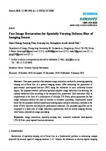
Fig. 2. Principle of the coarse-to-fine thresholded Landweber (CFTL) algorithm for a two-level decomposition.

for every , then inequality (5) holds for an arbitrary vector of wavelet coefficients satisfying the following constraint: there , . is a scale such that for all subbands Proof: Equality (9) reduces to

Combining this with the fact that, for every

, which couples the subbands). If the next itera, it is, however, not necessary to tion is performed at scale recompute the entire residual; instead, one can simply update . Denoting by the modificathe subbands tions that have been applied to the estimate, the corresponding correction that must be applied to the residual in a subband is

, (12)

we obtain

Appendix A describes an algorithm for computing the conin the convolutive case; for more general operators stants one may use the power method [49]. Let us emphasize that, under the condition of Property 1, every application of (10) is guaranteed to decrease the auxiliary functional (and, thus, the original cost functional), despite the fact that only a subset of subbands is updated. This follows from (7), which shows that the minimization of the auxiliary functional can always be divided into a collection of subband-specific—hence, independent—minimization problems. Of course, by letting vary at every iteration, we can successively update the subbands at all scales. The next section describes an efficient method for doing this. III. CONQUER—MULTILEVEL THRESHOLDED LANDWEBER ALGORITHM The general idea behind our multilevel scheme is to interlace the computation of the residual and the minimization procedure. To give the reader the intuition of this principle, we focus on the description of a simplified strategy that consists in applying (10) successively from the coarsest-scale to the finest-scale subbands. A. Coarse-to-Fine Update Strategy be the residual corresponding Let is modified at scale to the current estimate. Assume that by applying procedure (10). In general, this will imply a modification of the residual in all subbands (due to the matrix

The above equality stems from the cascade implementation of the wavelet transform—see (4). Thus, an updated version of the is obtained as follows: residual at scale 1) transfer all modifications to the scaling-function subband ; at the next finer scale 2) apply the “correction matrices” for every ; 3) subtract the results from the respective subbands. This principle is illustrated in Fig. 2; its recursive application leads to the “coarse-to-fine thresholded Landweber” (CFTL) algorithm. A pseudo-code description is given below. Note that all modifications—including those from subbands located at coarser scales than the current scale —are progressively transfered to finer scales. The CFTL algorithm depends on the “single-level thresholded Landweber” (SLTL) procedure, which essentially corresponds to the updating rule (10). The only difference is that the modifications that are applied to the estimate are stored in intermediate variables so as to be able , to update the residual. For simplicity, the variables and are considered to be global (for every subband ) in all pseudo-code descriptions given in this paper. We emphasize that the correction steps 2) and 3) above are the only additional operations compared to the standard TL algorithm. These steps should require little computational effort at coarse levels, thanks to the pyramidal structure of (decimated) wavelet representations. In other words, they can be implemented efficiently if the computational complexity of (the forward image-formation model followed evaluating by the corresponding “back-projection”) scales well with this data-size reduction. is a convolution matrix. A particular case arises when The shift-invariant structure of wavelet subspaces then implies that the correction steps essentially reduce to filtering operations. Here we refer to Appendix A, which also gives a recursive method for precomputing the correction filters: the procedure



is akin to a wavelet decomposition of the convolution kernel and is easily implementable in the frecorresponding to quency domain (see also [50]). The correction steps can be implemented with a linear cost provided that we store the DFTs of the individual wavelet subbands; the actual wavelet coefficients are only needed for the thresholding operations and can be computed efficiently using the FFT algorithm. In terms of computational work, one iteration of our algorithm is, therefore, equivalent to two FFTs per subband, which amounts to two FFTs at the signal level (level 0). The overall complexity of a full coarse-to-fine run is, thus, on the same order as one run of the standard TL algorithm, which also requires two FFTs per iteration in the convolutive case. With a slight anticipation of the next subsection, we conclude this part by noting that multigrid methodologies sometimes advocate the approximate resolution of coarse-level problems [15]. In the particular situations where the wavelet subbands are weakly coupled by the image-formation operator, we have indeed observed that the CFTL algorithm converges even if the correction steps are not applied; that is, if the residual is only updated at the beginning of the iteration loop. This amounts to applying (8) using fairly optimistic bound constants—without guarantee that the cost functional is monotonically decreased—and calls for further investigation. This approach may turn out to be useful when dealing with complex image-formation models that can not be evaluated easily at coarse levels. Algorithm 1 For every • • •

:

Algorithm 2 CFTL

• Initialization: — Choose some initial estimate — Compute its wavelet decomposition: • Repeat times: — Compute the residual: for every

,

— Update the subbands from coarse to fine levels, i.e., for , : • Update the subbands at the current level: • Transfer the modifications to the next finer level: • If , correct the residual for the wavelet subbands at the next finer level: , for every — Set • Return

515

B. General Multilevel Scheme With the previous algorithm in mind, one can conceive of more general multilevel strategies for updating the different scales in a more flexible manner. In Appendix B, we provide a pseudo-code description of a method that is strongly inspired by the multigrid paradigm. However, there is one fundamental difference: traditional multigrid schemes typically cycle through nested subspaces corresponding to increasingly coarse discretizations of the original inverse problem [51]. In the present context, we successively update the wavelet subbands at every scale; that is, we reinterpret the different scales of the wavelet transform as a multilevel representation of the inverse problem. The corresponding subspaces are not nested—they contain the oscillating components corresponding to the difference between successive coarse-level approximations. Incidentally, early attempts to apply the multigrid paradigm to image-restoration problems remained relatively unsuccessful because they were concentrating on slowly oscillating components [52], [53]. We have tried to specify the “multilevel thresholded Landweber” (MLTL) algorithm in a modular way that is relatively close to machine implementation. Its main building block, UpdateLevel , depends on three parameters so as to be able to mimic typical multigrid schemes (see Fig. 3). and , following The parameters are, thus, named , the conventions of the multigrid literature [15], [54]. In the , and , one retrieves the particular case coarse-to-fine update described in the preceding subsection [Fig. 3(a)]. However, we should note that the MLTL algorithm is numerically (slightly) more stable, because the current estimate is explicitely reconstructed from its wavelet coefficients at every iteration. The different modules of Appendix B can be summarized as follows. • UpdateResidual : updates the residual for the subbands at scale (if needed). Uses the correction principle of Fig. 2 if the wavelet subbands have not been modified so far. Otherwise, the update is performed by temporarily moving up to the next finer scaling-function subband. • UpdateLevel : recursive procedure which — updates the subbands at coarser scales by calling itself times; (the — updates the subbands at scale by calling number of updates before and after a recursive call are and , respectively). fixed by Note that the procedure must compute the current residual for the scaling-function subband at scale before calling itself. This is either done by applying the correction principle of Fig. 2 in the opposite direction (from the wavelet subbands to the scaling-function subband), or by going to the next finer scale using UpdateResidual . • MLTL: main routine that performs initialization tasks followed by several iterations of the update procedure. One may devise even more general—e.g. “full multigrid” [14]—schemes by adapting this routine. C. Fixed-Point Property A comprehensive study of the convergence properties of the MLTL algorithm is well beyond the scope of the present work.


516


The characterization of Property 2 is equivalent to the folsuch that, for every lowing statement: there is a component of either or

Fig. 3. Examples of multigrid-like updating schemes made possible by the general MLTL algorithm. Each dot corresponds to an application of (10) at the corresponding level. (a) Coarse-to-fine ( ; ; ); (b) V-cycles ; ); (c) W-cycles ( ; ). (

In particular, obtaining tight theoretical convergence-rate estimates is a difficult problem even for linear subspace-correction methods [51]. In the next section, we thus propose a numerical study of the convergence rate of the MLTL algorithm, based on the following concise characterization of the minimizer(s) of the cost functional (1). We provide a proof in Appendix C for completeness (see also [8] and the general results in [40] and [55]). is a minimizer of if and only if it is a Property 2: fixed point of the standard TL algorithm, that is, if and only if such that there is an arbitrary step size . Furthermore the minimizer is unique is positive definite. if A similar property can be obtained for the MLTL algorithm. This ensures that we obtain a minimizer of the cost functional whenever the MLTL algorithm converges (which is essentially guaranteed by the monotonicity of the algorithm [21]). In the stands for the th component of a vector . sequel, Property 3: is a minimizer of if and only if it is a fixed point of the MLTL algorithm; that is, if and only if it is not modified by a sequence of successive applications of (10) at different scales, such that every subband is updated at least once. Proof: is assumed to be a minimizer of . • Necessary part:

and and

(13) Multiplying by a suitable constant shows that the step size can actually be chosen arbitrarily. In particular, if corresponds to a wavelet coefficient of subband , (13) . Using this argument for all wavelet also holds for coefficients shows that is a fixed point of (10) at any scale . is assumed to be invariant under a se• Sufficient part: quence of successive applications of (10), such that every scale is visited at least once. We first observe that, for a given scale , (10) computes the minimizer of the auxiliary functional considered as only. Because this minimizer is a function of unique, the result of applying (10) is either to leave the estimate unchanged, or to strictly decrease the auxiliary functional—and, thus, the original cost functional by construction. The fixed-point assumption excludes the latter case. Thereis invariant under each individual fore, it must be that , application of (10). Let be an arbitrary component of . Since we assume e.g. corresponding to a subband that (10) was applied at scale at least once, (13) holds ; in fact, it holds for an arbitrary . Using with this argument for all wavelet coefficients, one retrieves the characterization of Property 2. Before proceeding to the experimental part of this work, we mention two straightforward extensions of the MLTL algorithm. First, it is clear that the algorithm (and the above results) can be extended to a cost functional with subband-specific regularization parameters . In particular, the coarsest-scale saling-funcis not thresholded in practice, i.e., . tion subband Second, one can also replace the -regularization in (1) by another coefficient-wise penalization in the wavelet-domain. This will essentially amount to changing the thresholding function; as long as the regularization term is convex, the same bound-optimization framework can be deployed. IV. NUMERICAL EXPERIMENTS In the experiments presented below, we use an norm for the regularization term. Unless specified otherwise, we use the same regularization parameter for all wavelet subbands; the scalingfunction subband is never penalized. A. Asymptotic Convergence (1-D Experiments) To evaluate the convergence behavior of the MLTL algorithm, we designed an experiment where the true minimizer of the cost functional is used as a gold standard. Each test case was constructed as follows. The standard “bumps” signal [Fig. 4(a)] is convolved with an -periodic low-pass kernel for ; defined by is normalized such the corresponding convolution matrix



that . White Gaussian noise is added to the result, so as to simulate a measurement . The standard TL ) is then initialized with this algorithm (with a step size measurement and run for 50000 iterations in order to obtain our . Since is positive-definite reference solution for the convolution kernel defined above (the smallest DFT being 0.06), Property 2 implies that this coefficient of minimizer is unique. Fig. 4(b) and (c) shows an example of the measurement and of the corresponding minimizer . Fig. 4(d) shows the locations of the nonzero wavelet coefficients of the solution (we use a 3-level wavelet decomposition and the upper plot represents the finest-resolution subband). We then used this reference to compare the asymptotic behavior of the TL and MLTL algorithms. To this end, we performed a series of experiments where the algorithms are applied to the minimization of (1) and initialized with the measurement . Although the asymptotic convergence rates that are presented here may not be directly relevant to practical situations, they give a quantitative indication of the acceleration potential of the MLTL algorithm. Our asymptotic study required several thousand iterations of the TL and MLTL algorithms in various configurations, which is why we resorted to a small-scale problem and ). The MLTL algorithm was used with the ( parameters , and (coarse-to-fine strategy). The computational cost of one complete MLTL iteration is then essentially the same as the cost of one TL iteration (each subband is updated once per iteration). This allows for a direct comparison of both algorithms in terms of number of iterations. The decay of the cost functional towards its minimal value is represented in Fig. 4(e). This decay is only limited by the numerical precision of the computer environment (we used Matlab on a 64-bit Intel Xeon workstation). To reach this limit with the MLTL algorithm, the number of iterations is divided by more than 10 compared to the TL algorithm. We also display the distance between the estimate and the minimizer [Fig. 4(f)]; here, the “signal-to-error-ratio gain” is defined as . As expected, both algorithms converge to the minimizer, but the MLTL algorithm is again faster by more than one order of magnitude for reaching the level of numerical precision. To obtain a more quantitative insight, we repeated the experiment in several test cases and computed the slope of the SERG curves between 100 and 250 dB. This measurement gives an estimate of the asymptotic convergence rate, in dB per iteration. The results are summarized in Table I, for various orthonormal wavelet bases and different values of the regularization parameter, corresponding to different noise levels (from top to bottom, the values of correspond to BSNR noise levels of 60, 50, 40, 30, 20, 10 dB, respectively—see [12] for the definition of BSNR). For validation purposes, we computed a theoretical conver. With this particular gence-rate estimate in the case where choice, both algorithms reduce to linear (least squares) restoration procedures: since the thresholding step disappears, the TL algorithm reduces to the standard Landweber iteration and the MLTL algorithm corresponds to a wavelet-based multilevel implementation of the Landweber iteration. For this type of linear iterations, the asymptotic convergence rate can be estimated

Fig. 4. Experiment with a known minimizer (Symlet8, inal signal ; (b) measurement ; (c) minimizer coefficients of ; (e) cost function:

517

). (a) Orig; (d) active wavelet ; (f) SERG (dB).

using the spectral radius of the so-called iteration matrix (see e.g. [54]). This spectral radius can be obtained directly for the TL algorithm because we consider orthonormal wavelet bases


518


TABLE I CONVERGENCE RATES (IN dB PER ITERATION) FOR DIFFERENT VALUES OF THE REGULARIZATION PARAMETER AND VARIOUS ORTHONORMAL WAVELET BASES

(the computation is essentially the same as in Section II-C). For the MLTL algorithm, the small dimension of the problem allows us to explicitly construct the iteration matrix in order to evaluate its spectral radius. The resulting theoretical convergence-rate estimates (expressed in dB per iteration for comparison purposes) are reported in the first row of Table I. The theoretical and the measured values are in good agree, suggesting that our experimental method for ment for measuring the asymptotic convergence rate is reliable. The recorroborate the former observation [7], [12] that sults for the TL algorithm tends to converge faster for higher values of . This can be explained by the fact that the variational problem is more constrained, thus compensating for the unfavorable conditioning of the convolution kernel. Nevertheless, the convergence rates of the MLTL algorithm are consistently one order of magnitude larger than those of the TL algorithm. The figures suggest that the strongest acceleration is generally obtained for higher-order wavelets, which can be related to their improved frequency selectivity. The Shannon wavelet basis provides perfect frequency selectivity, a property that was exploited in our previous work [12]. B. Computation Time (2-D Experiments) In our second series of experiments, we evaluated the performance of the MLTL algorithm in terms of computation time. This type of assessment is most relevant in practical situations, but it depends on computer hardware parameters. Therefore, we always provide a comparison with the standard TL algorithm. We first simulated the effect of a defocusing blur on a 512 512 test image [Fig. 5(a)]. We used a standard diffraction-limited point spread function (PSF) model for widefield fluorescence microscopy [1]. The result was then corrupted by additive white Gaussian noise with a BSNR of 40 dB [Fig. 5(b)]. We restored this simulated measurement using the

TL and MLTL algorithms. Both were initialized with the measurement. We used a separable orthonormalized cubic spline wavelet basis with four decomposition levels. The regularizawas the same for both algorithms; it was tion parameter adjusted using multiple trials, so as to give the best restoration quality after the MLTL algorithm had converged. Fig. 5(d) and (e) show the evolution of the restoration quality measure , where stands for the original signal and is the estimate. One can observe that the coarse-to-fine MLTL algorithm requires 1 s of computations to reach an improvement of 8 dB [result shown in Fig. 5(c)]. The TL algorithm needs approximately 10 s to reach the same figure. We found that the performance of the MLTL algorithm can be further improved by using , i.e., with a modified W-cycle iteration. This makes sense since natural images tend to have mostly low-frequency content; thus, iterating on coarse-scale subbands brings the largest improvement in the beginning, unless the algorithm is initialized with a very accurate estimate. We used a similar protocol for the second part of our 2-D experiments, where we replicated the standard test case used by Figueiredo and Nowak in [7] (Cameraman image convolved with a 9 9 uniform blur; additive white Gaussian noise with a BSNR of 40 dB; initialization with a Wiener-type estimate). In particular, we introduced a random shift of the estimate at the beginning of every TL and MLTL iteration; the authors found that this method gave optimal results with nontranslation-invariant wavelet transforms. We present results for three wavelet bases, including biorthogonal 9/7 wavelets. We always used three decomposition levels and the same regularization . The second and fourth columns of Table II parameter show the restoration quality of the MLTL algorithm after 1 and 4 s, respectively. The third and fifth columns give the minimum TL computation time that is required to reach the same restoration quality. Again, the MLTL algorithm provides



519

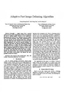
confirm the superiority of the Haar basis among separable wavelet bases for 2-D image restoration; this fact is already known from denoising applications [56]. In general, the ability to use other wavelet bases than the Shannon wavelet basis leads to substantial improvements over our previous work [12]. In summary, the MLTL algorithm can yield state-of-the-art results (similar to those obtained in [7]) in a substantially shorter time than the TL algorithm. C. Application to Real Fluorescence-Microscopy Data (3-D Experiments) To conclude this experimental part, we applied the MLTL algorithm to real 3-D fluorescence-microscopy data. Similarly to our experiment in [12], we acquired two image-stacks of the same sample (a C. Elegans embryo), one of them serving as a visual reference to assess the restoration quality. For the present work we acquired a much larger, two-channel data set. Both data sets were acquired on a confocal microscope, which has the ability to reject out-of-focus light using a small aperture in front of the detector. This creates a relatively sharp but noisy image [Fig. 6(d)]. When the aperture is opened the signal intensity is improved, but the measurement gets blurred by the contributions of defocused objects. This results in hazy images that are characteristic for widefield microscopes [Fig. 6(a)]. We applied the MLTL algorithm to the widefield-type stack, with three decomposition levels. To account for the anisotropic sampling scheme of the microscope, we used an orthonormalized linear spline wavelet for the X-Y dimensions, and a a Haar wavelet for the Z dimension. We kept the random-shift method of [7] and we used scale-dependent regularization parameters that were adjusted with the confocal stack as a visual reference. The channels were processed independently, using computer-generated PSFs based on a 3-D version of the diffraction-limited model used in the previous subsection. The parameters of this model were adjusted according to manufacturer-provided specifications of the objective, the immersion oil and the fluorescent dyes (NA, refractive index, emission wavelength). The result is shown in Fig. 6(c): the restored image-stack provides significantly better contrast than the original widefield image, especially for the filaments (green channel). The chromosomes and their centromeres (blue channel) appear almost as sharp as in the confocal image. For completeness, we have included the result of the TL algorithm after the same number of iterations [Fig. 6(b)]. It is seen that the resulting image-stack is still very hazy; the TL algorithm fails to produce a visible deconvolution effect within the assigned budget of iterations. The computation time was on the order of 5 minutes for both algorithms. V. DISCUSSION AND CONCLUSION

Fig. 5. Computation time comparison (in seconds). (a) Original; (b) measured; (c) restored (MLTL after 1 sec.); (d) SERG versus computation time; (e) SERG versus computation time (zoom).

an acceleration of roughly one order of magnitude. Our results

We have presented a wavelet-based multilevel image-restoration algorithm inspired from multigrid techniques. The method is one order of magnitude faster than the standard algorithm for sparsity-constrained restoration, whose results belong to the state-of-the-art in the field of image processing. The MLTL algorithm allows for typical multigrid iteration schemes such as V-cycles and W-cycles. However, it differs from textbook multigrid schemes, which iterate on nested


520


TABLE II COMPUTATION TIME REQUIRED TO REACH A GIVEN LEVEL OF RESTORATION QUALITY, FOR THE SECOND EXPERIMENT OF SECTION IV-B

subspaces corresponding to different “resolution levels” of the inverse problem. Our algorithm, by contrast, iterates on the wavelet subbands, which are the complements of the standard multigrid spaces. Yet our algorithm takes advantage of the underlying multiresolution structure, which greatly contributes to the efficiency of the method. The other key point is the preconditioning effect of wavelets. We have provided theoretical convergence rates for the linear parts of the TL and MLTL algorithms, giving a quantitative insight into the convergence acceleration of the latter. Our experimental results show that one can achieve the same kind of acceleration in the general nonlinear case (with thresholding). Our method is directly applicable to separable wavelet bases in arbitrary dimensions. We obtained promising results in the context of 3-D fluorescence microscopy using such bases, extending our previous work [12]. Nevertheless we have tried to provide a sufficiently general description that should require little adaptation for more “exotic” wavelet representations, e.g. with quincunx subsampling schemes [57], or nonstationary refinement filters [58], [59]. The algorithm is readily implementable using our modular specification and standard wavelet-decomposition/reconstruction building blocks. We are currently investigating the benefits of the MLTL algorithm for redundant wavelet representations. We have not specifically explored this possibility here because we were primarily interested in high-dimensional inverse problems that do typically not allow for redundant decompositions. We have already obtained promising results for medical applications (specifically fMRI signal restoration and tomographic image reconstruction) which will be the subject of forthcoming reports. APPENDIX A. A Method for Precomputing the Bound Constants and the Correction Filters To keep the presentation simple, we will consider the 1-D situation where is a (positive) circulant matrix. Its eigenvalues (DFT coefficients) are real and positive and can , . Furthermore, we will thus be denoted consider a wavelet decomposition with a dyadic subsampling scheme. The method presented below can easily be extended to higher dimensions and more general wavelet representations. To compute the bound constants defined in (11), one must essentially estimate the inner products of (12). These can be rewritten in the frequency domain as

where we use the following conventions. denotes the DFT of the wavelet coefficients corre• sponding to a subband at a given level . Since we assume a dyadic subsampling scheme, can be seen as -periodic sequence, with . an • denotes the DFT of the wavelet or scaling function that spans the subspace associated with subband . Note , the discrete version of the that if we define standard scaling relation [26] can be stated as (14) where is the -periodic filter corresponding to (see below). Our multilevel method only requires the explicit value of the when and are subbands located at the same constants for some . In this case, level, that is, when and have the same period . We can thus write that

where

(15) Inequality (12) is then obtained by defining . is a circulant matrix and , the matrix When is also circulant and its DFT coefficients , for . This property are precisely given by allows for an efficient frequency-domain implementation of the residual correction steps in the CFTL and MLTL algorithms. To prove the property, we introduce the general notation for arbitrary subbands , . We . We can then proceed by recurrence. also define , is circulant and its DFT coefficients are given For by (15) with . For , we assume that is a circulant matrix whose DFT coefficients are . The cascade structure of the wavelet representation (4) implies that, for



521

For a given subband , the algorithmic interpretation of is . Its 1) dyadic upsampling, followed by 2) filtering with stands for 1) filtering with , followed by transpose 2) dyadic downsampling. Therefore, is also a circulant matrix with DFT coefficients

(16) , and from The equality stems from definition (15) for the scaling relation (14); this completes the proof by recurrence. Note that relation (16) provides a way to recursively compute and the corresponding constants (with the filters ). B. Pseudo-Code Description of the General MLTL Algorithm As in the previous subsection, we use the notation . The general MLTL algorithm uses both the and , for . It is useful to obmatrices : in the convolutive case, this implies that serve that . Algorithm 3 UpdateResidual • If for some : — — For every , : for every • Otherwise, if

. ,

.

Algorithm 4 UpdateLevel • Initialization: , . — For every , — For every • Repeat times: — Repeat times: • UpdateResidual . • SLTL . : — If • If for some : , UpdateResidual . • If • Otherwise, . • • UpdateLevel . . • times: — Repeat • UpdateResidual . • SLTL . . •

.

.

Fig. 6. Three-dimensional deconvolution results (maximum-intensity projections of image stacks). (a) Original widefield stack (input data); (b) deconvolution result after 15 TL iterations; (c) deconvolution result after 15 MLTL iterations; (d) confocal reference stack.

Algorithm 5 MLTL • Initialization: — Choose some initial estimate

and set

.

— Compute its wavelet decomposition (keeping the coarse approximations): , for every , for .


522


• Repeat times: . — — UpdateLevel(1). • Set and return .

REFERENCES

C. Proof of Property 2 A short computation reveals that

(17) where and are arbitrary vectors of wavelet coefficients. for every • Necessary part: we assume that . for — Suppose that some . Given a real and strictly positive constant , we define the vector by if otherwise. In view of (17), can always be chosen such that , a contradiction. Therefore, it must be that for every . and inserting into — Choosing (17) gives the necessary condition

If it were true that , we could find a sufficiently small such that this necessary condition is violated. Thus, it must be . that Since for every , it follows that whenever . The combination of both results is equivalent to the fixedpoint property. is assumed to be a fixed point of the TL • Sufficient part: algorithm. We use the same equivalence: — Since whenever , we know that and (17) reduces to

— Since follows that

for every , it

This also shows the unicity of the minimizer when is positive definite.

[1] C. Vonesch, F. Aguet, J.-L. Vonesch, and M. Unser, “The colored revolution of bioimaging,” IEEE Signal Process. Mag., vol. 23, no. 3, pp. 20–31, May 2006. [2] P. Sarder and A. Nehorai, “Deconvolution methods for 3-D fluorescence microscopy images,” IEEE Signal Process. Mag., vol. 23, no. 3, pp. 32–45, May 2006. [3] A. K. Louis, “Medical imaging: State of the art and future development,” Inv. Probl., vol. 8, no. 5, pp. 709–738, Oct. 1992. [4] Handbook of Medical Imaging: Physics and Psychophysics, J. Beutel, H. L. Kundel, and R. L. Van Metter, Eds. Bellingham, WA: SPIE, Feb. 2000, vol. 1. [5] R. Molina, J. Nunez, F. J. Cortijo, and J. Mateos, “Image restoration in astronomy: A Bayesian perspective,” IEEE Signal Process. Mag., vol. 18, no. 2, pp. 11–29, Mar. 2001. [6] J. L. Starck, E. Pantin, and F. Murtagh, “Deconvolution in astronomy: A review,” Pub. Astron. Soc. Pacific, vol. 114, no. 800, pp. 1051–1069, Oct. 2002. [7] M. A. T. Figueiredoa and R. D. Nowak, “An EM algorithm for waveletbased image restoration,” IEEE Trans. Image Process., vol. 12, no. 8, pp. 906–916, Aug. 2003. [8] I. Daubechies, M. Defrise, and C. De Mol, “An iterative thresholding algorithm for linear inverse problems with a sparsity constraint,” Commun. Pure Appl. Math., vol. 57, no. 11, pp. 1413–1457, Aug. 2004. [9] J. Bect, L. Blanc-Féraud, G. Aubert, and A. Chambolle, “A -unified variational framework for image restoration,” in Proc. ECCV, 2004, vol. 3024, pp. 1–13, Part IV. [10] I. Loris, G. Nolet, I. Daubechies, and F. A. Dahlen, “Tomographic inversion using -regularization of wavelet coefficients,” Geophys. J. Int., vol. 170, no. 1, pp. 359–370, July 2007. [11] J. M. Bioucas-Dias and M. A. T. Figueiredo, “A new TwIST: Twostep iterative shrinkage/thresholding algorithms for image restoration,” IEEE Trans. Image Process., vol. 16, no. 12, pp. 2992–3004, Dec. 2007. [12] C. Vonesch and M. Unser, “A fast thresholded Landweber algorithm for wavelet-regularized multidimensional deconvolution,” IEEE Trans. Image Process., vol. 17, no. 4, pp. 539–549, Apr. 2008. [13] S. Mallat, “A theory for multiresolution signal decomposition: The wavelet representation,” IEEE Trans. Pattern Anal. Mach. Intell., vol. 11, no. 7, pp. 674–693, Jul. 1989. [14] W. Hackbusch, Multi-Grid Methods and Applications. Berlin, Germany: Springer-Verlag, 1985, vol. 4, Springer Ser. Comput. Math. [15] W. L. Briggs, V. E. Henson, and S. F. McCormick, A Multigrid Tutorial, 2nd ed. Philadelphia, PA: SIAM, 2000. [16] W. M. Lawton, “Multiresolution properties of the wavelet Galerkin operator,” J. Math. Phys., vol. 32, no. 6, pp. 1440–1443, June 1991. [17] Z. Cai and W. E, “Hierarchical method for elliptic problems using wavelet,” Commun. Appl. Numer. Meth., vol. 8, no. 11, pp. 819–825, Nov. 1992. [18] W. Dahmen and A. Kunoth, “Multilevel preconditioning,” Numer. Math., vol. 63, no. 1, pp. 315–344, Dec. 1992. [19] W. L. Briggs and V. E. Henson, “Wavelets and multigrid,” SIAM J. Sci. Comput., vol. 14, no. 2, pp. 506–510, Mar. 1993. [20] G. Wang, J. Zhang, and G.-W. Pan, “Solution of inverse problems in image processing by wavelet expansion,” IEEE Trans. Image Process., vol. 4, no. 5, pp. 579–593, May 1995. [21] K. Lange, D. R. Hunter, and I. Yang, “Optimization transfer using surrogate objective functions,” J. Comput. Graph. Statist., vol. 9, no. 1, pp. 1–20, Mar. 2000. [22] D. R. Hunter and K. Lange, “A tutorial on MM algorithms,” Amer. Statist., vol. 58, no. 1, pp. 30–37, Feb. 2004. [23] M. W. Jacobson and J. A. Fessler, “An expanded theoretical treatment of iteration-dependent majorize-minimize algorithms,” IEEE Trans. Image Process., vol. 16, no. 10, pp. 2411–2422, Oct. 2007. [24] J. A. Fessler and A. O. Hero, “Space-alternating generalized expectation-maximization algorithm,” IEEE Trans. Signal Process., vol. 42, no. 10, pp. 2664–2677, Oct. 1994. [25] S. Oh, A. B. Milstein, C. A. Bouman, and K. J. Webb, “A general framework for nonlinear multigrid inversion,” IEEE Trans. Image Process., vol. 14, no. 1, pp. 125–140, Jan. 2005. [26] S. Mallat, A Wavelet Tour of Signal Processing. New York: Academic, 1998. [27] H. Yserentant, “On the multi-level splitting of finite element spaces,” Numer. Math., vol. 49, pp. 379–412, 1986.



[28] R. E. Bank, T. F. Dupont, and H. Yserentant, “The hierarchical basis multigrid method,” Numer. Math., vol. 52, no. 4, pp. 427–458, Jul. 1988. [29] P. S. Vassilevski and J. Wang, “Stabilizing the hierarchical basis by approximate wavelets I: Theory,” Numer. Lin. Algebra Appl., vol. 4, no. 2, pp. 103–126, Mar./Apr. 1998. [30] M. Bertero and P. Boccacci, Introduction to Inverse Problems in Imaging. Bristol, U.K.: IOP, 1998. [31] C. Christopoulos, A. Skodras, and T. Ebrahimi, “The JPEG2000 still image coding system: An overview,” IEEE Trans. Consum. Electron., vol. 46, no. 4, pp. 1103–1127, Nov. 2000. [32] C. De Mol and M. Defrise, “A note on wavelet-based inversion algorithms,” in Inverse Problems, Image Analysis and Medical Imaging, M. Z. Nashed and O. Scherzer, Eds. Providence, RI: American Mathematical Society, Nov. 2002, vol. 313, Contemporary Mathematics, pp. 85–96, (Special Session on Interaction of Inverse Problems and Image Analysis. AMS Joint Mathematics Meetings, New Orleans, LA, Jan. 10–13, 2001). [33] R. D. Nowak and M. A. T. Figueiredo, “Fast wavelet-based image deconvolution using the EM algorithm,” presented at the 35th Asilomar Conf. Signals, Systems and Computers, Pacific Grove, CA, Nov. 2001. [34] J. L. Starck, D. L. Donoho, and E. J. Candès, “Astronomical image representation by the curvelet transform,” Astron. Astrophys., vol. 398, no. 2, pp. 785–800, February 2003. [35] J.-L. Starck, M. K. Nguyen, and F. Murtagh, “Wavelets and curvelets for image deconvolution: A combined approach,” Signal Process., vol. 83, no. 10, pp. 2279–2283, October 2003. [36] L. Landweber, “An iterative formula for Fredholm integral equations of the first kind,” Amer. J. Math., vol. 73, no. 3, pp. 615–624, Jul. 1951. [37] J. B. Weaver, Y. S. Xu, D. M. Healy, and L. D. Cromwell, “Filtering noise from images with wavelet transforms,” Magn. Res. Med., vol. 21, no. 2, pp. 288–295, Oct. 1991. [38] D. L. Donoho, “De-noising by soft-thresholding,” IEEE Trans. Inf. Theory, vol. 41, no. 3, pp. 613–627, May 1995. [39] M. Liebling and M. Unser, “Autofocus for digital fresnel holograms by use of a fresnelet-sparsity criterion,” J. Opt. Soc. Amer. A, vol. 21, no. 12, pp. 2424–2430, Dec. 2004. [40] C. Chaux, P. L. Combettes, J.-C. Pesquet, and V. R. Wajs, “A variational formulation for frame-based inverse problems,” Inv. Probl., vol. 23, no. 4, pp. 1495–1518, Aug. 2007. [41] J. M. Bioucas-Dias, “Bayesian wavelet-based image deconvolution: A GEM algorithm exploiting a class of heavy-tailed priors,” IEEE Trans. Image Process., vol. 15, no. 4, pp. 937–951, Apr. 2006. [42] M. A. T. Figueiredo, J. M. Bioucas-Dias, and R. D. Nowak, “Majorization-minimization algorithms for wavelet-based image restoration,” IEEE Trans. Image Process., vol. 16, no. 12, pp. 2980–2991, Dec. 2007. [43] M. Elad, “Why simple shrinkage is still relevant for redundant representations?,” IEEE Trans. Inf. Theory, vol. 52, no. 12, pp. 5559–5569, Dec. 2006. [44] M. Elad, B. Matalon, and M. Zibulevsky, “Coordinate and subspace optimization methods for linear least squares with non-quadratic regularization,” Appl. Comput. Harmon. Anal., vol. 23, no. 3, pp. 346–367, Nov. 2007. [45] M. A. T. Figueiredo, R. D. Nowak, and S. J. Wright, “Gradient projection for sparse reconstruction: Application to compressed sensing and other inverse problems,” IEEE J. Sel. Topics Signal Process., vol. 2007, no. 4, pp. 586–597, Dec. 2007. [46] J. Friedman, T. Hastie, H. Höfling, and R. Tibshirani, “Pathwise coordinate optimization,” Ann. Appl. Statist., vol. 1, no. 2, pp. 302–332, Dec. 2007. [47] M. Fornasier, “Domain decomposition methods for linear inverse problems with sparsity constraints,” Inv. Probl., vol. 23, no. 6, pp. 2505–2526, Dec. 2007. [48] A. Chambolle, R. A. DeVore, N.-Y. Lee, and B. J. Lucier, “Nonlinear wavelet image processing: Variational problems, compression, and noise removal through wavelet shrinkage,” IEEE Trans. Image Process., vol. 7, no. 3, pp. 319–335, Mar. 1998. [49] G. H. Golub and C. F. van Loan, Matrix Computations. Baltimore, MD: Johns Hopkins Univ. Press, 1996.

523

[50] T. Blu and M. Unser, “The fractional spline wavelet transform: Definition and implementation,” in Proc. 25th IEEE Int. Conf. Acoust., Speech, Signal Process., Jun. 2000, vol. I, pp. 512–515. [51] J. Xu, “The method of subspace corrections,” J. Comput. Appl. Math., vol. 128, no. 1–2, pp. 335–362, Mar. 2001. [52] K. Zhou and C. K. Rushforth, “Image restoration using multigrid methods,” Appl. Opt., vol. 30, no. 20, pp. 2906–2912, Jul. 1991. [53] T.-S. Pan and A. E. Yagle, “Numerical study of multigrid implementations of some iterative image reconstruction algorithms,” IEEE Trans. Med. Imag., vol. 10, no. 4, pp. 572–288, Dec. 1991. [54] W. Hackbusch, Iterative Solution of Large Sparse Systems of Equations. New York: Springer-Verlag, 1994, vol. 95, Appl. Math. Sci. [55] P. L. Combettes and V. R. Wajs, “Signal recovery by proximal forward-backward splitting,” Multiscale Model. Simul., vol. 4, no. 4, pp. 1168–1200, 2005. [56] T. Blu and F. Luisier, “The SURE-LET approach to image denoising,” IEEE Trans. Image Process., vol. 16, no. 11, pp. 2778–2786, Nov. 2007. [57] D. van de Ville, T. Blu, and M. Unser, “Isotropic polyharmonic B-splines: Scaling functions and wavelets,” IEEE Trans. Image Process., vol. 14, no. 11, pp. 1798–1813, Nov. 2005. [58] I. Khalidov and M. Unser, “From differential equations to the construction of new wavelet-like bases,” IEEE Trans. Signal Process., vol. 54, no. 4, pp. 1256–1267, Apr. 2006. [59] C. Vonesch, T. Blu, and M. Unser, “Generalized Daubechies wavelet families,” IEEE Trans. Signal Process., vol. 55, no. 9, pp. 4415–4429, Sep. 2007.

Cédric Vonesch was born on April 14, 1981, in Obernai, France. He spent one year studying at the Ecole Nationale Supérieure des Télécommunications, Paris, France, and graduated from the Swiss Institute of Technology, Lausanne (EPFL), in 2004, where he is currently pursuing the Ph.D. degree. He is currently with the Biomedical Imaging Group, EPFL. His research interests include multiresolution and wavelet analysis, inverse problems, and applications to bioimaging.

Michael Unser (M’89–M’94–F’99) received the M.S. (summa cum laude) and Ph.D. degrees in electrical engineering in 1981 and 1984, respectively, from the Ecole Polytechnique Fédérale de Lausanne (EPFL), Switzerland. From 1985 to 1997, he was a Scientist with the National Institutes of Health, Bethesda, MD. He is now a Full Professor and Director of the Biomedical Imaging Group at the EPFL. His main research area is biomedical image processing. He has a strong interest in sampling theories, multiresolution algorithms, wavelets, and the use of splines for image processing. He has published over 150 journal papers on those topics, and is one of ISIs Highly Cited authors in Engineering (http://isihighlycited.com). Dr. Unser has held the position of associate Editor-in-Chief (2003–2005) of the IEEE TRANSACTIONS ON MEDICAL IMAGING, for which he also served as an Associate Editor (1999–2002, 2006–2007). He has also served as an Associate Editor for the IEEE TRANSACTIONS ON IMAGE PROCESSING (1992–1995) and the IEEE SIGNAL PROCESSING LETTERS (1994–1998). He is currently a member of the editorial boards of Foundations and Trends in Signal Processing, the SIAM Journal of Imaging Sciences, and Sampling Theory in Signal and Image Processing. He co-organized the first IEEE International Symposium on Biomedical Imaging (ISBI 2002). He was the founding chair of the technical committee of the IEEE-SP Society on Bio Imaging and Signal Processing (BISP). He received the 1995 and 2003 Best Paper Awards and the 2000 Magazine Award from the IEEE Signal Processing Society.


A Fast Multilevel Algorithm for Wavelet-Regularized Image Restoration

A Fast Multilevel Algorithm for Wavelet-Regularized Image Restoration

Suggest Documents

a multilevel fast multipole algorithm for analyzing

A Hardware Algorithm for Fast Realistic Image

A fast multilevel algorithm for graph clustering and ... - Semantic Scholar

A multilevel domain decomposition algorithm for fast O(N ... - InstaRecon

A forward-backward algorithm for image restoration with ... - spars'05

Fast FCM Algorithm for brain MR Image

Fast pairwise nearest neighbor based algorithm for multilevel ...

A Fast Hierarchical Multilevel Image Segmentation Method using ...

Improved variational image registration model and a fast algorithm for ...

A Fast Learning Algorithm for Image Segmentation with Max-Pooling

A Fast Convex Hull Algorithm for Binary Image

CAAM Technical Report TR07-10 A Fast Algorithm for Image

a fast algorithm for digital image scaling - CiteSeerX

A Fast B-Spline Pseudo-inversion Algorithm for Consistent Image ...

A fast wavelet algorithm for image deblurring - Semantic Scholar

A Fast Algorithm for Image Super-Resolution from

Pixel Intensity Clustering Algorithm for Multilevel Image Segmentation

Modified Discrete Grey Wolf Optimizer Algorithm for Multilevel Image ...

Fast Image Restoration Methods for Impulse and ... - Google Sites

Fast Image Restoration for Spatially Varying Defocus Blur of ... - MDPI

Fast Image Restoration Methods for Impulse and ... - Google Sites

Blurred image restoration: A fast method of finding ... - Semantic Scholar

Parallel ProXimal Algorithm for Image Restoration Using Hybrid ...

Adaptive Fast Image Dehazing Algorithm - IEEE Xplore