a Fast Sparse Triangular Solve with Sparse Level Tile Layout on ...

swSpTRSV: a Fast Sparse Triangular Solve with Sparse Level Tile Layout on Sunway Architectures Xinliang Wang

Weifeng Liu

Department of Computer Science and Technology Tsinghua University, China [email protected]

Department of Computer Science Norwegian University of Science and Technology, Norway [email protected]

Wei Xue

Li Wu



Abstract

ACM Reference Format: Xinliang Wang, Weifeng Liu, Wei Xue, and Li Wu. 2018. swSpTRSV: a Fast Sparse Triangular Solve with Sparse Level Tile Layout on Sunway Architectures. In PPoPP ’18: Principles and Practice of Parallel Programming, February 24–28, 2018, Vienna, Austria. ACM, New York, NY, USA, 16 pages. https://doi.org/10.1145/3178487.3178513

Sparse triangular solve (SpTRSV) is one of the most important kernels in many real-world applications. Currently, much research on parallel SpTRSV focuses on level-set construction for reducing the number of inter-level synchronizations. However, the out-of-control data reuse and high cost for global memory or shared cache access in inter-level synchronization have been largely neglected in existing work. In this paper, we propose a novel data layout called Sparse Level Tile to make all data reuse under control, and design a Producer-Consumer pairing method to make any inter-level synchronization only happen in very fast register communication. We implement our data layout and algorithms on an SW26010 many-core processor, which is the main buildingblock of the current world fastest supercomputer Sunway Taihulight. The experimental results of testing all 2057 square matrices from the Florida Matrix Collection show that our method achieves an average speedup of 6.9 and the best speedup of 38.5 over parallel level-set method. Our method also outperforms the latest methods on a KNC many-core processor in 1856 matrices and the latest methods on a K80 GPU in 1672 matrices, respectively.

1

Introduction

The sparse triangular solve (SpTRSV) operation computes a solution vector x for a linear system Lx = b1 , where L is a sparse lower triangular matrix and b is a right-hand side vector. The SpTRSV operation is in general indispensable to the solve phase of sparse direct solvers [11] and preconditioners of sparse iterative solvers [44] in a wide range of applications from numerical simulation [42] to machine learning [35]. Unlike other sparse basic linear algebra subprograms [28] such as sparse transposition [60], sparse matrix-vector multiplication [31, 33] and sparse matrix-matrix multiplication [32], the SpTRSV is an inherently sequential operation. In worst cases (e.g., when L is a triangular double-band matrix), any solution component x i , if i , 0, needs to wait for its former components to solve out. This makes parallelizing SpTRSV seem not possible. But by grouping components without dependencies between each other into one set, SpTRSV can run in parallel. Although multiple sets have to run level-by-level (i.e., in serial, because of the dependencies between their components), at least the components inside a set can be calculated simultaneously. This is so-called level-set method first presented by Anderson and Saad [2] and Saltz [45], and recently improved by Park et al. [40] and Liu et al. [29]. The total overheads for the level-set methods are two-fold: the calculation cost inside each level and the synchronization cost between one level to another. The proportions of the two parts highly depend on the sparsity structure of input matrix.

CCS Concepts • Theory of computation → Parallel algorithms; Keywords Sparse matrix, Sparse triangular solve, Sparse level tile, Sunway architecture Permission to make digital or hard copies of all or part of this work for personal or classroom use is granted without fee provided that copies are not made or distributed for profit or commercial advantage and that copies bear this notice and the full citation on the first page. Copyrights for components of this work owned by others than the author(s) must be honored. Abstracting with credit is permitted. To copy otherwise, or republish, to post on servers or to redistribute to lists, requires prior specific permission and/or a fee. Request permissions from [email protected]. PPoPP ’18, February 24–28, 2018, Vienna, Austria © 2018 Copyright held by the owner/author(s). Publication rights licensed to the Association for Computing Machinery. ACM ISBN 978-1-4503-4982-6/18/02. . . $15.00 https://doi.org/10.1145/3178487.3178513

1 Here

we only use lower triangular matrix for problem formulation. But note that any discussion in this paper can be easily ported to solve an upper triangular system Ux = b.

338

PPoPP ’18, February 24–28, 2018, Vienna, Austria

Xinliang Wang, Weifeng Liu, Wei Xue, and Li Wu makes cores in the same column share x through register communication but not global memory. All 2057 square matrices from the Florida Sparse Matrix Collection [8] are tested to evaluate the performance of our proposed method and the latest approaches running on Intel Xeon Phi (KNC) and Nvidia K80 GPU. Compared with the parallel level-set method on SW26010, our algorithm achieves an average speedup of 6.9 and a maximal speedup of 38.5. Our method also outperforms the latest methods on KNC in 1856 benchmarks and the latest methods on K80 in 1672 benchmarks, respectively. The paper makes the following contributions: • The Sparse Level Tile layout is proposed to make data reuse of vectors x and b under control and to make their memory access coarse-grained, predictable and prefetchable. • A Producer-Consumer pairing method is designed to make any inter-level synchronization only happen through very fast register communication but not slow global memory. • Totally 2057 sparse matrices are used for performance evaluation, in which our method largely outperforms parallel level-set methods and the latest methods on KNC and GPU.

Unfortunately, in most real-world matrices (as collected in the University of Florida Sparse Matrix Collection [8]), the synchronization cost dominates the overall execution time. This makes the performance of parallel SpTRSV through the level-set methods far from satisfactory. Compared to sparse matrix-vector multiplication (SpMV) [31, 33, 58, 64], the SpTRSV kernel has exactly the same calculation cost (in term of the amount of arithmetic and memory accessing operations) but can be up to over a hundred times slower than SpMV on modern processors [23, 25, 29, 30]. Based on a comprehensive study, Li and Saad [25] pointed out that SpTRSV is the actual performance bottleneck of parallel preconditioned iterative solvers, due to the high cost of interlevel synchronization. Even though recent research (e.g., sparsifying synchronization by pruning [40] and replacing synchronization by atomic operations [29]) improved level-set method through reducing the amount of synchronization, it has not explored the potential of memory subsystems of modern processors. This underexploration is reflected in two aspects: (1) data reuse of x and b overly relies on cache, which is hardware managed and may not supply the best data swapping; and (2) inter-level synchronization, even of the recently proposed methods [29, 40], needs to go through shared global memory, which is too slow compared to inter-core communication. Our proposed method is primarily concerned with parallel SpTRSV aware of data locality and fast synchronization. Besides the parallelism, which has been already developed by the level-set methods, we further tap the potential from memory access for higher performance. We propose a new data layout called Sparse Level Tile, or SLT for short, to divide a sparse matrix into two types of 2D tiles with nonuniformed shapes. By carefully establishing the connections between these tiles, the SLT layout gives highly efficient data reuse for both solution x and right-hand side b, and migrates the fine-grained, random and unprefetchable memory access to coarse-grained, predictable and prefetchable. As for fast synchronization, we best exploit the inter-core communication of the newly developed SW26010 many-core processor, which is the main building-block of the current world fastest supercomputer Sunway Taihulight (125 Pflops peak performance, 93 Pflops sustained LINPACK performance, composed of 40960 SW26010 processors [1]). The processor offers a register communication scheme that works in the same row or column of its cores in a 2D mesh. This regular communication pattern offers opportunities for fast inter-core communication but also challenges the irregular sparse matrix problems we are facing. Based on the relationship between x i and bi , we design a Producer-Consumer pairing method, where the paired x i and bi are held in the paired Producer and Consumer respectively. The paired Producer and Consumer are in the same row which makes any inter-level synchronization only happen through register communication in the same row. Meanwhile, such method

2

Background and Motivation

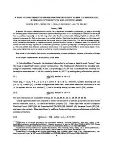
2.1 Serial Algorithm for SpTRSV Alg.1 lists a serial algorithm for Lx = b2 . As can be seen, there is no naïve concurrency in the outer for loop (line 1), due to the dependency between each element of x and its previous elements (line 4). Taking the problem in the left half of Fig.1 as an example3 , x 0 , x 2 and x 3 cannot be solved in parallel, since x 3 depends on x 0 and x 2 to solve out first. Algorithm 1 A serial SpTRSV algorithm for Lx = b. Input: L of size n × n, b of size n; Output: x of size n; 1: for j = 0 to n − 1 do 2: x j = b j /l j j 3: for each l i j on column j of L do 4: bi = bi − l i j x j 5: end for 6: end for

2.2 Level-Set Methods for Parallel SpTRSV Luckily, some potential concurrency can be exploited in this problem with careful analysis. For example, x 3 – x 8 can be calculated concurrently after x 0 – x 2 are completed. Based on this discovery, parallelizable components x 0 – x 2 , x 3 – x 8 , x 9 – x 13 , x 14 – x 15 are grouped into four sets, and a dependency graph composed of four levels (i.e., the four sets) can be 2 Here L can be stored in any format, though the compressed sparse column (CSC) layout may be better since Alg.1 is a column-wise algorithm. 3 Note that here the components in the levels are ordered in restrict ascending order. This is not typical in real-world problems. But doing so is helpful for describing our problems, and it is easy to reorder/permute matrix rows to this form when the level information is known.

339

swSpTRSV 0: 1: 2: 3: 4: 5: 6: 7: 8: 9: 10: 11: 12: 13: 14: 15:

PPoPP ’18, February 24–28, 2018, Vienna, Austria Thread 0

still high. The main reason is that inter-core synchronization has to go through global memories or low-level shared caches, both of which offer lower bandwidth and higher latency compared with high-level private caches and registers. Furthermore, as the number of cores goes up, the potential competition of accessing the global memory or shared cache between different cores often further hurts the performance.

Level 0

Thread 1

Thread 2

Level 1

Level 2

Level 3

2.4 Sunway Architecture The major building block of the supercomputer Sunway Taihulight is the SW26010 many-core processor, as shown in Fig.2. Each processor is composed of four Core Groups (CGs), and each CG contains a Management Processing Element (MPE) for latency sensitive tasks and one Computing Processing Element (CPE) cluster of 64 CPEs organized as an 8×8 mesh for throughput sensitive tasks. Each MPE has 32 KB L1 data cache and 256 KB L2 instruction/data cache, while each CPE has its own 16 KB L1 instruction cache and a 64 KB Scratch Pad Memory (SPM), whose speed is equal with that of L1 cache. A CG has 34.1 GB/s theoretical memory bandwidth and 765 GFlops double-precision peak performance [9, 13].

Figure 1. The left part shows a 16-by-16 sparse lower triangular matrix, and the right part plots four level-sets, corresponding dependency and the assignment to three threads.

extracted for parallel execution. The right half of Fig.1 shows the dependency graph of the level-set method. However, to make sure all the dependent elements have been calculated out, a synchronization (see the three dotted lines in the dependency graph in Fig.1) is introduced after each level’s computation. Unfortunately, on modern processors, especially many-core architectures, the cost for synchronization is expensive and sometimes dominates the execution time of parallel SpTRSV [25, 29, 40]. To reduce the costs for synchronization across threads, two approaches have been proposed. One method by Park et al. [40] replaces the full-synchronization with multiple corecore (P2P) synchronization. In the above example, the x 13 calculated by Thread 2 on level 2 only depends on the x 4 of Thread 0 and x 7 and x 8 of Thread 2 on level 1. Thus, a single P2P synchronization between Threads 0 and 2 is enough to guarantee correctness. Another optimization by Liu et al. [29] replaces synchronization with atomic operations. In Fig.1, Threads 0 and 2 on level 0 can update x 6 by atomically adding the results of x 0 and x 2 . Before the atomic-add is finished, Thread 1 busy-waits the lock on x 6 getting updated.

Main Memory M C M P E

M C M P E

CG

L1 L2

CPE Cluster

CG

Network on Chip (NoC)

SI M P E

CPE Cluster

M P E

CPE Cluster

M C

M C

CG

CG

Main Memory

Main Memory

CPE cluster CPE

CPE

CPE

CPE

CPE

CPE

CPE

CPE

CPE

CPE

CPE

CPE

CPE

CPE

CPE

8

8 CPE

SPM

Figure 2. The block diagram of an SW26010 processor.

2.3 Performance Problems in Existing Methods Traditional data layouts, such as CSR4 and CSC, are unaware of data reuse. As shown in line 4 of Alg.1, methods based on the CSC layout traverse the nonzeros in the column (vertical) direction, which leads to perfect data reuse of x but makes the reuse of b handled by hardware. Similar, methods based on the CSR layout traverse the nonzeros in the row (horizontal) direction, which leads to perfect reuse of b but makes the reuse of x out-of-control. Both methods only consider data reuse in one dimension. Thus, methods based on either of the two layouts may not achieve the best performance. Later on, we will design a new layout to carefully traverse the nonzeros in both row and column directions, i.e., in 2D space, and to make the reuse of x and b both under control. It is well known that the inter-level synchronization cost is expensive for parallel SpTRSV. Even though [40] and [29] have replaced full synchronization with P2P synchronization or atomic operations, the overhead for synchronization is 4 The

CPE Cluster

Main Memory

Two kinds of memory access, i.e., Direct Memory Access (DMA) and global load/store (Gload/Gstore), are supported, between which an obvious performance gap exists: DMA prefers transferring massive data from main memory to SPM, and Gload/Gstore prefers transferring small and random data between main memory and registers. A Stream Triad test [63] shows that the bandwidth of DMA and Gload/Gstore are 22.6 GB/s and 1.48 GB/s, respectively. The CPE cluster offers low-latency register data communication among the 8 × 8 CPEs, and this is one of the key features of the SW26010 processor. Each CPE has Register Send Buffer and Register Receive Buffer. The hardware will send data from one Send Buffer to another Receive Buffer uninterruptedly and automatically until the Send Buffer is empty or the Receive Buffer is full. According to the benchmarking results [63], the latency of the register communication is at most 11 cycles and the integrated core-core communication bandwidth is 637 GB/s. However, due to the limitation of the hardware, the data in register can only be communicated between the CPEs in the same row or column.

compressed sparse row format.

340

3

0

right-hand vector b

2

1

3

4

5

8 7 6 9 10 X-Region 0 X-Region 1 X-Region 2 X-Region 3

solution vector x

A

F B-Region 3 B-Region 2 B-Region 1 B-Region 0

0

Step 1

1

3 4

5 6 X-Region 0 X-Region 1 X-Region 2 X-Region 3

X-Region 0 X-Region 1 X-Region 2 X-Region 3

B L1

0

1 2 3

L2 4 5

L3

6

Sparse Level Tile Layout

E

Step 2 B-Region 3 B-Region 2 B-Region 1 B-Region 0

L0

Step 5

2

B-Region 3 B-Region 2 B-Region 1 B-Region 0

2.5 Challenges of SpTRSV on Sunway Architecture Even though the SPM can help us manually control the timing of data swapping for better reuse, and the register communication technique improves the efficiency of inter-core data-sharing and synchronization, it is still challenging to use these advantages for parallel SpTRSV. First, the fine-grained and unpredictable memory access of SpTRSV is unsuitable with the features of Sunway architecture. The fine-grained memory access can only use the Gload/Gstore method with low bandwidth and high latency, or use the DMA method in low efficiency. Meanwhile, the memory access of SpTRSV is unpredictable, which means that we need to estimate whether the data is cached or not before each load/store instruction. This is natural for hardware controlled caches but will cost much more for SPM, because the estimating process is done by software but not hardware. Furthermore, the unpredictable memory access also makes it impossible to prefetch any data. On the other hand, when parallelizing the SpTRSV, a CPE may need to synchronize to any other CPEs for sharing data or finishing dependencies. However, This cannot be directly supported by the register communication technique on Sunway processors, because such high-speed communication only works for CPEs in the same row or the same column. A straight forward idea is to select some CPEs as “transfer stations” to achieve register communication between those CPEs not in the same row/column. However, such method may introduce a cycle of messaging route, thus potential deadlock may occur [26].


Xinliang Wang, Weifeng Liu, Wei Xue, and Li Wu

0

Step 4

1

Step 3

2 3

4 5 6



C

D



In this section, we design a new data layout, called Sparse Level Tile (SLT for short) layout, to make the reuse of x and b both under control and to migrate the memory access of SpTRSV from fine-grained, random and unprefetchable to coarse-grained, predictable and prefetchable.

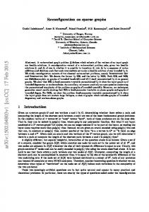
Figure 3. The establishing process for Sparse Level Tile layout. Based on Region, the x and b will be divided into X-Regions and B-Regions (B). The original levels will be separated into new levels if crossing Regions (C). Each nonzero belongs to a Diagonal-Tile (D) or an Offdiagonal-Tile (E) according to the ID of the used X-Region and modified B-Region. The Tiles modifying the same B-Region will be gathered together to improve the data reuse of b elements (F). The numbers in (F) denote tile order for both storing and computing.

3.1 Data Layout Design The key point of the SLT layout is to divide a triangular matrix into multiple Tiles, each of which only applies to part of x and b. Here, we use the general term “cache” as the fastest memory on different processors, meaning that for Sunway architecture, the “cache” is the SPM, and for other processors, the “cache” may be high-level cache. Fig.3 presents the establishing process of the SLT layout, where Fig.3A is the example matrix plotted in Fig.1 with four level-sets, and Fig.3B–Fig.3F are the output after each of the five steps described in the rest of this section. Step 1. Import the Concept of Region. We introduce a high-level concept named Region to divide both x and b, and then make X-Region and B-Region, respectively. Each

Tile uses x elements from some X-Regions to modify b elements from some B-Regions. The Region size is corresponding to the cache size. In the following steps, we will group the nonzeros into different Tiles to limit the number of XRegions and B-Regions that each Tile uses and modifies. In this example, we assume the Region size is 4 elements, which leads to 16/4 = 4 Regions for the 16 unknowns. As an example in Fig.3, the first off-diagonal nonzeros on the top-left (l 3,0 ) of Fig.3B uses x 0 from X-Region 0 (i.e., ⌊0/4⌋ = 0) to modify b3 from B-Region 0 (i.e., ⌊3/4⌋ = 0). Step 2. Separate Original Levels. A level is separated into multiple levels when going across more than one X-Regions. For example, the original L1 will be separated into three levels, as it crosses three X-Regions. Totally, the original four levels will be translated into seven levels. Note that

341

swSpTRSV 0

PPoPP ’18, February 24–28, 2018, Vienna, Austria 1

3 4

2

5 6

10

9

Inherit from previous Tile Load from main memory Obtained from Used in Inherit

8

7

Load from main memory Store to main memory

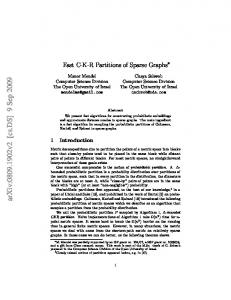
Figure 4. The dataflow using the SLT layout. Each bi will only be loaded once and will never be swapped out until it is used to compute x i (Line 2 in Alg.1). The nonzeros in two dimension in each Tile make x i be reused as much as possible. When targeting a Tile, all the corresponding data must be cached to guarantee predictability. The streaming access of x and b from main memory makes it possible to prefetch coarse-grainedly.

this operation usually introduces more levels to a problem. But since our method processes synchronizations in a very low-cost way, it is not sensitive to the number of level-sets. Step 3. Build Diagonal-Tiles. To improve the data reuse of x and b and to make memory access predictable, we combine the diagonal nonzeros of each level with their “nearest” off-diagonal nonzeros together to consist the first kind of Tiles, Diagonal-Tiles or DiaTiles for short. The width of a DiaTile is the number of diagonal nonzeros in each level, and the height is the width plus the Region size. Hence, the term “nearest” refers to a range that the DiaTile’s nonzeros should be in. The number of DiaTiles is equal to the number of divided levels. In our case, this number is seven. In the seven DiaTiles, all x elements inside one single Tile can be solved out without dependencies inside the current Tile, but only with dependencies from its previous Tiles. From the figure, it can be seen that a DiaTile is composed of a diagonal on top and a square matrix on the bottom, meaning that x elements corresponding to this diagonal can be together solved by x j = b j /l j j (if previous dependencies outside this Tile are released). This spatial feature actually decouples operations x j = b j /l j j (only for the diagonal on top) and bi = bi − li j x j (only for the square in the bottom) inside a single DiaTile. This makes tasks in a DiaTile work in a perfectly parallel-friendly way. It is worth to note that this is why we use this non-uniformed tiling instead of regular 2D tiling selected by previous work [5, 19, 37, 41, 62]. Taking the left most DiaTile in Fig.3D as an example, we can see that its width is 3 as there are three diagonal nonzeros, and the Region size is 4. So its height is 4 + 3 = 7. In this DiaTile, we can solve out x 0 , x 1 and x 2 , which must be cached. As the Region size is 4, only b3 , b4 , b5 and b6 are stored in cache. To make memory access predictable, which means that we can guarantee the corresponding x and b elements must be cached without any extra estimating, each nonzero in this Tile must have a row index smaller than heiдht = 7. Then, this Tile only uses X-Region 0 to modify B-Region 0 and B-Region 1. In this DiaTile, x 0 and x 2 can be reused

three times and twice respectively, as three and two nonzeros exist below. Similar, b3 and b6 , stored in the cache, can be reused twice as two nonzeros exist on the left, respectively. Note that the cached b elements will be updated by some bi = bi − li j x j operations (Line 4 of Alg.1), and can be reused when conducting the calculation within its following Tiles. Step 4. Build Offdiagonal-Tiles. Note that not all the off-diagonal nonzeros have been assigned to DiaTiles. We now need to group the rest of the nonzeros together to build another kind of Tile: Offdiagonal-Tile, or OffdiaTile for short. We let the nonzeros of an OffdiaTile only use a single X-Region and modify a single B-Region. As a result, both the maximal width and height of an OffdiaTile are equal with Region size. However, as some off-diagonal nonzeros have been assigned to DiaTiles, the actual range of an OffdiaTile might be smaller. Take the top-left OffdiaTile of the matrix (storing one nonzero) in Fig.3E as an example. This Tile uses X-Region 0 and modifies B-Region 1. Similar, the OffdiaTile located below the former OffdiaTile (storing six nonzeros) uses X-Region 0 and modifies B-Region 2. The goal of building OffdiaTile is to make memory access predictable and to improve data reuse. Before targeting an OffdiaTile, we can load a bunch of x and b elements, the size of which is equal to the Region size. As each OffdiaTile only uses a single X-Region and modifies a single B-Region, the corresponding x and b must be cached and can be reused. Step 5. Sort Tiles. We want to further improve the datareuse of b. The way is to closely store the Tiles modifying the same B-Region. Then we can only load part of a B-Region but not the whole B-Region before processing each Tile. Then a Tile, regardless it is Diagonal or Offdiagonal, belongs to a Region ID, which is the maximal ID of the B-Region it can modify. We will store Tiles according to their Region IDs. As can be seen in Fig.3F, because the potential maximal row index of Tile 1 is 7 and it can modify b7 from B-Region 1 (even though there are no nonzeros in this tile having a row index of 7), Tile 1 belongs to Region ⌊7/4⌋ = 1. In summary, Tiles 0, 1 and 2 belong to Region 1, Tiles 3 and 4 belong to

342



Region 2, Tiles 5, 6, 7 and 8 belong to Region 3, and Tiles 9 and 10 belong to Region 4 (The B-Region 4 cannot be found in Fig.3 since it locates beyond the matrix size and has no effect on solving process). For the Tiles belong to different Region IDs, Tiles belong to smaller IDs are stored in front of those belong to larger IDs. For Tiles belong to the same Region ID, DiaTiles are stored in front of OffdiaTiles and OffdiaTiles with the same Region ID can be stored in arbitrary order. The storing order of Tiles, as shown in Fig.3F, is same with the computing order. So we can load the Tiles in a stream.

converting process is fast. In our experiments, the conversion of large matrices in our benchmark requires up to several seconds. Further considering an SLT matrix can be used many times once created, the conversion cost is trivial. 3.3 SpTRSV Algorithm based on the SLT Layout To store a matrix using the SLT layout, six variables are needed: l, li, lj, tiles, sizes and idx, as exhibited in Alg.3. The l, li, lj stores the values, the row and column indices of the lower triangular matrix L respectively; The tiles stores the number of Tiles, including both Diagonal- and OffdiagonalTiles; The idx stores the index of the first nonzero of each Tile; The sizes stores the number of diagonal nonzeros for the DiaTiles and zero for OffdiaTiles. Line 10 computes x j = b j /l j j and Line 15 computes bi = bi − li j x j . The memory access to b and x in both Line 10 and 15 is predictable, because we can guarantee that the corresponding x and b elements have already been cached (cx and cb). The memory access to matrix L is also coarsegrained and prefectchable, because the Tiles are stored in the same order with that of computation, and we can load a whole Tile from the main memory before each kernel starts.

3.2 Dataflow, Data Reuse and Data Storage Fig.4 uses the example matrix in Fig.1 and Fig.3 for explaining dataflow and data reuse based on the SLT layout. Here we take Tiles 0, 1 and 2 as an example. Tile 0 only focuses on x 0 -x 2 and b3 -b6 . So we can guarantee that these data must be cached without any extra estimating when using Tile 0. x 0 is reused three times to modify b3 , b4 and b6 , and x 2 is reused twice to modify b3 and b6 . Similar, b3 and b6 are reused twice to be modified by x 0 and x 3 . After Tile 0 is finished, b3 -b6 are in the cache. So, when targeting Tile 1, x 3 is obtained by x 3 = b3 /l 3,3 , and b3 -b6 are inherited directly. Both of these two operations are in the cache. Thanks to the order well organized, only b7 are loaded from the main memory for Tile 1. Next, for Tile 2, x 0 -x 3 are reloaded from main memory and b4 -b7 can be inherited from Tile 1 directly and perfectly. The inheritance of b elements in this order can make us reuse b until they are transformed to x elements after x j = b j /l j j (Line 2 in Alg.1). It can also avoid any redundant memory access to b. Meanwhile, the nonzeros in two dimensions in each Tile can reuse the x elements as much as possible. When targeting a Tile, any memory access is predictable since the corresponding data must be cached. As the memory access to x and b for DiaTiles are in streaming, it can be guaranteed to prefetch b and integrally store x by introducing other on-chip buffers in implementation, and the memory access must be coarse-grained. Alg.2 presents the pseudocode that establishes the SLT layout. We first calculate the level-set information and separate the original level-sets into new levels, as introduced in Steps 1 and 2. Next, we traverse all the nonzeros to classify them into different Tiles, including Diagonal- and OffdiagonalTiles, as introduced in Steps 3 and 4. At last, we sort these tiles to improve the data-reuse, as motioned in Step 5. The layout of storing each Tile is flexible. Any sparse matrix representations, e.g., CSR, CSR or COO5 , are usable. To minimize redundant information, we select the COO as the low-level layout for each Tile and make the nonzeros inside each Tile ordered (this can be done by calling the parallel segmented sort kernel [16]). Also note that converting a matrix from another layout to the SLT layout mainly includes obtaining Tile information and moving nonzeros. Thus the 5 The

Algorithm 2 The pre-process for establishing SLT layout 1: function preprocess 2: //Compute original level information 3: //Separate original levels into new levels based on Regions 4: for i = 0 → #new _l evels − 1 do 5: for < r ow, col, val > ∈ new _l evels[i] do 6: if r ow < idx [i] + sizes[i] + REGI O N _S I Z E then 7: Diaдonal _T il e[i].add (< r ow, col, val >) 8: else 9: O f f diaдonal _T il e[ ⌊r ow /REGI O N _S I Z E ⌋] 10: [ ⌊col /REGI O N _S I Z E ⌋].add (< r ow, col, val >) 11: end if 12: end for 13: end for 14: //Sort Diaдonal _T il es and O f f diaдonal _T il es if not empty 15: end function

3.4 Tuning the Region Size in the SLT Layout The Region size in the SLT layout essentially affects the performance. Compared with large Region size, small Region size leads to more levels and more Offdiagonal-Tiles, the latter of which will reduce the x elements’ reuse and cause more extra reloading of x elements (Line 13 in Alg.3). While large Region size makes each targeting OffdiagonalTile reload a large amount of x elements. If the targeting Tile is very sparse, there will be lots of redundancy in these reloading x elements. According to our experiment, a small Region size suits problems with lots of levels thus few parallelism, while a large Region size suits problems with high parallelism. Detailed results can be found in Sec.5.3.

coordinate format stores row/col indices and value for each nonzero.

343

swSpTRSV


Algorithm 3 The SLT-based SpTRSV algorithm.

communication to replace full synchronization. This sending operation, together with corresponding x j = b j /l j j , is represented by the “x j = b j /l j j ” Line in Fig.4. Except the b elements sent out, other b elements are still in the cache_b, which is represented by the “Inherit” Line in Fig .4. Here, we introduce a concept owner for each x element, b element and nonzero. Each b element’s owner is a Consumer using the b element for bi = bi − ∆i j . Each x element’s owner is a Producer computing the x element by x j = b j /l j j , and Each nonzero’s owner is a Producer using the nonzero for x j = b j /l j j or ∆i j = li j x j . We first averagely distribute the b elements to all the Consumers. Due to the one-to-one pairing, we can further determine the owner of each x element in the same row simply. Therefore, we can successfully assign the owner for each x element, b element and diagonal nonzero. Next, we will assign each off-diagonal nonzero’s owner, to make sure the communication only happens in the same row or column. Observe that each bi = bi −li j x j , imported by the off-diagonal nonzero, uses x j to modify bi , and the owners of both x j and bi have been assigned. So we can distribute the nonzero to the Producer, which has the same column with the x j ’s owner, and the same row with the bi ’s owner. By such distributing method, each ∆ will be sent only by the Row register communication and each x element will be shared across the CPEs in the same column only by the Column register communication.

Input: l, li, l j, t il es, sizes, idx, b Output: x 1: function SpTRSV(x, b, l, li, l j, t il es, sizes, idx ) 2: CACHE cx [REGION_SIZE] // cache for x 3: CACHE cb[REGION_SIZE] // cache for b 4: Replenish cb from b for REGION_SIZE 5: for t = 0 → t il es − 1 do 6: nodnz ← idx [t + 1] − idx [t ] − sizes[t ] 7: if Tile is Diagonal then 8: Copy cb to cx for sizes[t ] 9: Replenish cb from b for sizes[t ] 10: Vector Division for sizes[t ] //x j = b j /l j j 11: Store cx to x for sizes[t ] 12: else if Tile is OffDiagonal then 13: Load x to cx for REGION_SIZE 14: end if 15: cb = cb − T il e t × cx for nodnz //bi = bi − l i j x j , T il e t means the submatrix consist of the nonzeros in Tile t 16: end for 17: end function

4

Implementation on Sunway architecture

4.1 Producer-Consumer Pairing Method In this subsection, we propose a Producer-Consumer pairing method to utilize the regular register communication pattern for our irregular problem. Fig.5 plots our method. For the whole CPE cluster, we define Producers as its left half part (i.e., 32 CPEs on the left) and Consumers as its right half part (i.e., the other 32 CPEs on the right). But note that we can also use a combination of 16-16, 8-8, or 4-4. Because the CPEs are organized as an 8 × 8 2D mesh, 8, 4, 2 or 1 rows of the mesh are used for the varied number of Producers/Consumers, respectively. The performance of tuning this number is discussed in Sec. 5.3. We can see that each diagonal nonzero of a triangular matrix imports x j = b j /l j j (Line 10 in Alg.3) and each off-diagonal nonzero imports bi = bi − li j x j (Line 15 in Alg.3), and each bi = bi − li j x j can be separated into ∆i j = li j x j and bi = bi − ∆i j . Then we have three kinds of operations and assign x j = b j /l j j and ∆i j = li j x j to Producers and bi = bi − ∆i j to Consumers. Each Producer has a cache_x and a buffer_l, the former one is used to cache and reuse x elements and the latter one is to coarse-grainedly prefetch the nonzeros in each Tile. Similarly, each Consumer has a cache_b and a buffer_b. The former one is used to cache and reuse b elements and the latter one is to coarse-grainedly prefetch b. In fact, both the cache and the buffer are part of the SPM. But in our design, only the data in cache can be reused, while the data in the buffer cannot, till moved from buffer to cache. Note that multiplying cache_b size on each Consumer and the number of Consumers is the Region size of the SLT layout. Each Producer will be paired with one Consumer. The b element in bi = bi − ∆i j on one Consumer is exactly needed by x j = b j /l j j on the paired Producer. So, before each level’s computation, Consumers will send corresponding b elements to their paired Producers using the Row register

4.2 SpTRSV with Producer-Consumer Pairing In this subsection, we introduce the solving process for both Diagonal-Tiles and Offdiagonal-Tiles, as exhibited in Fig.5B. Step 1. The Producers load the current Tile from the main memory to their buffer_l. Then all the CPEs check whether the current Tile is Diagonal. If the answer is ‘Yes’, the Consumers will send the b elements to their paired Producers by the Row register communication for reuse (2a). While, if the answer is ‘no’, the Producers will reload the x elements from the main memory directly to the cache_x. Step 2. If we are targeting a Diagonal-Tile, the Producers will finish the x j = b j /l j j and then store the x back to the main memory, and the Consumers will move the buffer_b’s b elements to their cache_b. The Consumers will replenish buffer_b once it is empty. Step 3. When the current Tile is ‘thin’ (which means the cache_x of each Producer is large enough to hold the x elements from all the Producers in the same column), the Producers will do a Whole-Rolling by the Column register communication to share their x elements to all the Producers in the same column (5a). Then Producers finish ∆i j = li j x j and send ∆ to corresponding Consumers by the Row register Communication (6a). The Consumers finally complete “bi = bi − ∆i j ” after getting the ∆.

344

PPoPP ’18, February 24–28, 2018, Vienna, Austria Send

from Consumers to Producers 2a

cache_b

Group

Producer-Consumer Pair 5a

;

8 rows

6b

A B C D Total

Consumers

Producers

cache_x

Xinliang Wang, Weifeng Liu, Wei Xue, and Li Wu Parallelism Range Average [20 , 25 ) 15.97 [25 , 210 ) 287.59 [210, 215 ) 7064.68 [215, 220 ) 358216.55 [20 , 220 ) 30010.37

#Matrices 249 1015 634 159 2057

Table 1. A statistics of the four groups of matrices tested.

Here we test all of the 2057 square matrices from the University of Florida Sparse Matrix Collection [8] (containing in total 2757 matrices: 700 rectangular and 2057 square matrices) to maximize the coverage of matrix features (i.e., matrix size, sparsity structure, the number of level-sets and application domains). Without loss of generality, we only execute lower triangular solve for each matrix, and add a major diagonal to make it nonsingular. To better visualize the large amount of results recorded, we divide the 2057 matrices into four groups according to their parallelism. Here, as work [29, 40] already did, we define the term parallelism as the average number of nonzeros per level (i.e., nnz/#levels). Tab.1 lists a statistics of the four groups of matrices.

4 columns

buffer_l

Send

from Producers to Consumers 5b 6a

A

buffer_b

Start 1: Load Tile into buffer_l;

2a: Producers recieve to cache_x from Consumers;

Y

2b: Reload

3: Producers compute and store to main memory; 4: Consumers move from buffer_b to cache_b; 5b: Producers compute and send to Consumers;

6b: Sub-Roll in the same column;

Diagonal-Tile?

N

N

into cache_x;

Tile is thin?

Y

5a: Whole-Roll in the same column;

Y

1.E+2

#Cycles < CPEs rows

6a: Producers compute and send to Consumers;

B

1.E+1

Inspector Time (s)

N

End

1.E+0

Figure 5. The Producer-Consumer pairing method and solving process on Sunway architecture. Each Producer will be paired with one Consumer, and the synchronization before each level’s computation will only happen in each pair. The Producers in the same column will share x elements using Column register communication. The numbers 2a, 5a, 5b, 6a and 6b in subfigure A are the related operations in subfigure B.

1.E-2 1.E-3 1.E-4 1.E+1

1.E+2

1.E+3

1.E+4

1.E+5

1.E+6

1.E+7

1.E+8

Number of nonzeros

Figure 6. The inspector cost for all the matrices. The cheapest cost is 0.0003s, and the most expensive cost is 28.1621s. The harmonic average is 0.0033s

Step 4. If the current Tile is not ‘thin’, each Producer does a Sub-Rolling to send cached x elements to its lower neighbour and receive new x elements from its upper neighbour by Column register communication to replace its cached x elements (6b), after consuming all the nonzeros based on its cached x elements (5b). We need to make each x element cross all the Producers in the same column, so this step needs to be repeated multiple times (named as Cycle for short), and the times equal with the number of CPE rows we adopt. The only reason of having this Step is that the cache_x has a limited size and may not hold all the data at the same time. In summary, thanks to the Producer-Consumer pairing method, we complete inter-level synchronization and data sharing by very fast Row/Column register communication.

5

1.E-1

The three platforms are equipped with an SW26010 processor, an Nvidia Tesla K80 GPU, and an Intel Xeon Phi (KNC) processor, respectively. We test three SpTRSV methods (i.e., serial code, parallel level-set method, and the proposed swSpTRSV) on the SW26010 processor, three GPU methods (i.e., cuSparse 8.0 SpTRSV v1 and v2, and SyncFree [29]) and two x86 methods from Intel (i.e., serial/parallel MKL and P2P [40]). Note that to achieve the best performance, we test the above algorithms on the processors they designed for. Also, if a device has multiple “work nodes”, we only use one of them. Specifically, a work node of an SW26010 is one of its four CGs, and of an Nvidia K80 GPU is one of its two GK210 chips. Tab.2 lists more details. Also note that the experiments are completed in double precision, and each performance number is the average of 200 runs.

Experimental Results

5.1 Experimental Setup To benchmark our proposed algorithm and existing methods, we evaluate 2057 sparse matrices on three platforms.

5.2 The Cost of establishing SLT layout Fig.6 presents the cost of establishing SLT layout for all 2057 benchmarks. The cheapest cost is 0.0003 s, occurs in the

345

swSpTRSV


The processors A single CG of an SW26010 (1 MPE + 64 CPEs @ 1.45GHz, 8 GB DDR3 @ 34.1 GB/s) A single chip of an NVIDIA K80 (1 GK210, 2496 CUDA cores @ 875 MHz, 12 GB GDDR5 @ 240 GB/s) An Intel Xeon Phi 7120 (61 x86 cores with 244 hyper-threads @ 1.33GHz, 16 GB DDR5 @ 352 GB/s)

The participating SpTRSV algorithms (1) A sequential SpTRSV on MPE. (2) A basic parallel level-set SpTRSV on CPEs. (3) The parallel swSpTRSV method proposed in this paper on CPEs. (1) The SpTRSV methods v1 (i.e., cusparse?csrsv) in NVIDIA cuSparse v8.0. (2) The SpTRSV methods v2 (i.e., cusparse?csrsv2) in NVIDIA cuSparse v8.0. (3) The synchronization-free method proposed by Liu et al. [29]. (1) The best performance of serial and parallel MKL SpTRSV (i.e., mkl_?csrtrsv and mkl_sparse_?_trsv) in MKL 2017 update 3. (2) The P2P synchronization method by Park et al. [40].

Table 2. The testbeds and participating SpTRSV algorithms Group A

Group B

Group C

4x8=32

2x8=16

2x8=16

1x8=8

1x8=8 128

256

512 1024 2048 4096

4x8=32 2x8=16 1x8=8

128

Size of cache_b (elements in double)

Group D

8x8=64

Number of CPEs

4x8=32

Number of CPEs

8x8=64

Number of CPEs

Number of CPEs

8x8=64

256

512 1024 2048 4096

4x8=32 2x8=16 1x8=8

128


8x8=64

256

512 1024 2048 4096

128


256

1 0.9 0.8 0.7 0.6 0.5 0.4 0.3 0.2 0.1 0

512 1024 2048 4096


Figure 7. The impact of tuning the number of CPEs (i.e., the number of Producers/Consumers, see Sec. 4.1) and the size of cache_b (see Sec. 3.4). Each matrix is tested with 24 (4 × 6) parameter settings. Each value filled in the heat maps is a harmonic mean, this mean is calculated from ratios of the performance of current parameter setting to the highest performance of the 24 settings of all matrices in a group. 6

10

5

8

4

6

Actual size / Theoretical size

12

6

6

5

5

4

4

3

3

3

4

2

2

2

2

1

1

1

0

1x8=8 CPEs 2x8=16 CPEs 4x8=32 CPEs 8x8=64 CPES

0 1

2

4

8

16

32

0 32

64

128

256

512

1024

0

1024

2048

4096

8192

16384

32768

32768

65536 131072 262144 524288 1048576

Parallelism (nnz/levels) Figure 8. The ratio of actual amount of memory access to the theoretical amount of memory access. The former is calculated from our counters inserted into the code, and the latter is always Size(L) + Size(b) + Size(x).

matrix ‘Tina_DisCog’, while the most expensive cost is 28.16 s, occurs in the matrix ‘europe_osm’. The harmonic average of all costs is 0.0033 s. It can be seen that the cost is basically linear with the number of nonzeros, and most costs (68.8%) are between 0.001 s and 0.1 s. So in practice, establishing SLT layout is quite fast, especially when considering an SLT matrix can be used many times once created.

settings. For each of the four group, we calculate a normalized performance for one parameter setting. The results are illustrated in Fig.7. As can be seen, with the increase of parallelism, best throughput tends to be obtained by more CPEs and larger cache_b. For Group A, the best performance occurs at the point when #CPEs is 16 and cache_b is 256; For Group B, a combination of 32 CPEs and cache_b = 2048 achieves the best performance; And for Groups C and D, using all CPEs with 4096 entries in each cache_b is the best. It can also be seen in Fig.7 that the influence of tuning the number of CPEs is more significant than tuning cache_b size, in particular for the groups with less parallelism. So, we fix the cache_b size to the best, and adjust the number of CPEs to find more insights of where the performance differences come. By profiling the code with all 2057 matrices, we find that the ratio of the actual and the theoretical amount of memory access (both in Bytes) is the key issue here. We plot the metric in Fig.8. As can be seen, in Group A, the ratio is pretty high (up to about 12) when using 32 or 64

5.3 Effect of Parameter Tuning Note that multiplying #Producers or #Consumers and the size of cache_b is the Region size in the SLT layout. Thus, as described in Sec. 3.4 and Sec. 4.1, tuning the two parameters, i.e., #CPEs (2× #Producers or #Consumers) and the size of cache_b on each Consumer, may bring varied performance. To tune them for best performance, we exhaustively execute different combinations of the two parameters. We set #CPEs to {8, 16, 32, 64} and cache_b to {128, 256, 512, 1024, 2048, 4096}, and run all 2057 matrices with those 24 parameter

346

Performance (MFlops)

PPoPP ’18, February 24–28, 2018, Vienna, Austria 240

1200

200

1000

160

Xinliang Wang, Weifeng Liu, Wei Xue, and Li Wu 3600

3600

3000

3000

800

2400

2400

120

600

1800

1800

80

400

1200

1200

40

200

600

600

0

1

2

4

8

16

32

0

Serial Method on MPE Level-set Method on CPEs swSpTRSV on CPEs

32

64

128

256

512

0

1024

1024

2048

4096

8192

16384

32768

0

32768

65536

131072 262144 524288 1048576

Parallelism (nnz/levels) Figure 9. The performance of different methods on Sunway architecture. Compared with the serial method and the parallel level-set method, our parallel method obtains an average speedup of 7.8 (maximal speedup of 117.3) and an average speed of 6.9 (maximal speedup of 38.5), respectively.

Performance (MFlops)

240

MKL P2P cuSparse v1 cuSparse v2 SyncFree swSpTRSV

200 160 120 80 40 0

1

2

4

8

16

32

1200

6000

18000

1000

5000

15000

800

4000

12000

600

3000

9000

400

2000

6000

200

1000

3000

0

32

64

128

256

512

0

1024

1024

2048

4096

8192

16384

32768

0

32768

65536 131072 262144 524288 1048576

Parallelism (nnz/levels) Figure 10. The performance of different methods on different devices. Our method achieves the best performance in 1624 benchmarks.

parallelism increases to 32 and beyond (i.e., Groups B, C and D), our swSpTRSV can achieve noticeably higher performance. The poor performance of parallel level-set method is because of frequent, fine-grained and random memory access for x, which can only use Gload/Gstore. Thus level-set method’s performance may be even worse than the serial method in some cases. With the increase of parallelism, the performance gap between swSpTRSV and the other two methods is larger. Compared with the serial method, our method achieves an average speedup of 7.79 and the best speedup 117.3, occurs in matrix ‘kron_g500-logn21’ (n = 2M, nnz = 93M, #levels = 4340, parallelism=21460). Compared with the level-set method, our method obtains an average speedup of 6.9 and the best speedup 38.5, occurs in matrix ‘torso1’ (n = 116K, nnz = 4.5M, #levels = 1689, parallelism=2672). Tab.3 presents the power information of 20 typical benchmarks. The parallelism range from 21 to 669K. The power consist of two parts: the ddr power and the core power, the former of which reflects the energy cost of memory access and the latter reflects the cost of computation. With the increasing of the performance, both the ddr power, the core power, together with the performance/power increase. For the benchmark ‘net150’, where we obtain the highest performance, the total power reach 38.18 Watt and the performance/power is 89.22 MFlops/W. However, for the last three benchmarks, the power is high but the performance is low. This is because that there are lots of Offdiagonal-Tiles, which need much more memory access and obstruct high

CPEs. According to some other performance counters (not shown here for brevity), the extra memory accesses are from loading SLT information to more CPEs, and also from more frequently reloading x elements for Offdiagonal-Tiles. Thus, for matrices in Group A, 16 CPEs are enough to behave the best. With the increase of parallelism, the ratio becomes smaller. For Group B, the ratios of using 32, 16 or 8 CPEs are comparable (gradually become 1). More CPEs bring more parallel resource thus achieve better performance. Therefore, using 32 CPEs is the best. As for matrices in Groups C and D, the ratios of using different number of CPEs are almost identical (i.e., 1). Hence, using all the CPEs achieves the best performance due to higher parallelism. We will use the performance with the best group-wise (but not matrix-wise) parameter settings in the rest of the paper. In other words, for each matrix, we select the best parameter setting of the group it belongs to, regardless whether the setting brings the best performance for this single matrix. 5.4 Methods on Sunway Processor Here we compared the peformance of three methods on SW architecture: serial SpTRSV on one MPE, parallel level-set method and the proposed method on the 64 CPEs. Note that for the level-set method, memory access are set to go through the best paths, i.e., DMA for accessing L and b, and Gload/Gstore for accessing x, due to its randomness. The results are presented in Fig.9. For the benchmarks from Group A, swSpTRSV has comparable performance with the serial method, due to the poor parallelism and more memory accesses for the SLT layout information. But when the

347

swSpTRSV


name

#rows

#nonzeros

parallelism

dwt_1007 nemeth08 oscil_dcop_01 adder_dcop_02 cavity17 g7jac040 California barth qc2534 t3dh para-5 torso1 barrier2-1 atmosmodl kron_g500-logn21 net150 transient hugetrace-00010 patents circuit5M_dc

1007 9506 430 1813 4562 11790 9664 6691 2534 79171 155924 116158 113076 1489752 2097152 43520 178866 12057441 3774768 3523317

4791 202161 1027 5577 72685 71658 19751 21482 232947 2215638 2786141 4512480 1959072 5904756 93138084 1582360 570398 30139620 18744796 10631719

40 21 103 398 241 787 2195 1652 1201 1284 1445 2672 1672 13668 21460 395590 38027 174217 669457 38660

performance (MFlops) 102 146 181 300 415 651 760 872 1041 1129 1175 1269 1229 1514 2228 3406 1203 146 729 449

ddr idle (W) 4.29 4.29 4.29 4.29 4.29 4.29 4.29 4.29 4.29 4.29 4.29 4.29 4.29 4.29 4.29 4.29 4.29 4.29 4.29 4.29

core idle (W) 16.09 16.09 16.09 16.09 16.09 16.09 16.09 16.09 16.09 16.09 16.09 16.09 16.09 16.09 16.09 16.09 16.09 16.09 16.09 16.09

ddr (W) 4.69 4.49 5.09 5.09 4.99 5.49 6.19 6.09 5.79 5.79 5.89 6.09 5.89 6.89 7.69 8.79 6.99 6.89 6.99 6.99

core (W) 23.04 22.54 23.04 23.04 23.54 23.79 24.79 25.04 24.29 24.79 24.54 24.54 24.54 26.04 27.04 29.39 26.04 25.54 26.04 25.54

total (W) 27.73 27.03 28.13 28.13 28.53 29.28 30.98 31.13 30.08 30.58 30.43 30.63 30.43 32.93 34.73 38.18 33.03 32.43 33.03 32.53

performance/power (MFlops/W) 3.68 5.40 6.44 10.67 14.55 22.24 24.54 28.02 34.61 36.93 38.62 41.44 40.39 45.98 64.16 89.22 36.43 4.50 22.07 13.80

Table 3. The power of 20 typical benchmarks. The ddr power reflects the energy cost of memory access and the core power reflects the cost of computation.

performance. What reflects in the table is that the ddr power is high and does not matches the low core power.

MKL P2P cuSparse v1 cuSparse v2 SyncFree swSpTRSV Total

Group A 24 0 0 0 0 225 249

Group B 0 3 0 10 0 1002 1015

Group C 0 49 66 143 0 376 634

Group D 0 25 107 6 0 21 159

In summary, as listed in Tab.4, for all of the 2057 benchmarks, our method outperforms MKL and P2P methods on KNC in 1856 cases, and cuSparse and SyncFree methods on K80 in 1672 benchmarks. Totally, our method can achieve the best performance in 1624 matrices. It is worth to note that although the SyncFree method outperforms cuSparse v1 and v2 methods in many cases, it never demonstartes the best performance in the four Groups A–D. The reason is that its performance is lower than our swSpTRSV method in the low-parallelism benchmarks and is also lower than cuSparse v1 and v2 methods in the high-parallelism benchmarks. Though we list the performance of the recent work on various platforms, it is worth to note that this brief comparison may only guide algorithm design (which is the primary target of this work) within a certain range, due to dramatic architectural difference between the three platforms and their distinct design objectives for power-performance tradeoff.

Sum 24 77 173 159 0 1624 2057

Table 4. A statistics of the behavior of each method, in terms of the #matrices with the best performance achieved by it.

5.5 Different Methods on Different Processors We compare swSpTRSV with five recent SpTRSV methods developed for KNC Xeon Phi and K80 GPU. The performance is presented in Fig.10, and a statistics about the number of best performance achieved by each method is listed in Tab.4. In Group A, the MKL (serial) method has comparable performance with ours, and both of them are faster than the other implementations. The reason is that less parallelism brings more synchronizations, which makes parallel methods slow. But the serial MKL function does not suffer from synchronizations cost, and our method is not so sensitive to the number of synchronizations. When the parallelism increases, in Group B (containing around half of the tested matrices), swSpTRSV largely outperforms any other methods, thanks to the SLT layout and the low-cost synchronization techniques. For the matrices in Groups C and D, as the parallelism increases, the synchronization cost is relatively lower, and the calculation cost gradually dominates the overall cost. As a result, the compute pattern of SpTRSV is more like SpMV. Hence, GPU with more concurrent threads (which are very helpful for latency hiding) in general behaves the best.

6

Related Work

Concurrent data structures are fundamental building blocks for computer science. Data layout for better spatial locality and concurrency is becoming ever more crucial in the multiand many-core era [6, 10, 15, 22, 34, 36, 43, 53, 61, 68, 69]. Im and Yelick presented a register blocking method to improve the performance of SpMV [17]. Vuduc et al. demonstrated that well-designed data layouts for cache/register data reuse in SpMV operation provides superior performance [58], and similar optimization techniques are effective to serial SpTRSV operation as well [56, 59]. Strout et al. proposed sparse tiling [48, 49] that brings data locality and extra parallelism from both intra- and inter-iteration, and such techniques can also be extended to compile-time [47, 50] for automatically generating efficient code running in the inspector-executor mode [7]. Liu and Vinter [31] proposed the CSR5 storage

348



format for avoiding degraded SpMV performance due to the irregularity of the distribution of nonzero entries. Moreover, because of the diversity of sparsity structures, recent research [24, 52, 70] suggested to analyze nonzero layout and select the best sparse kernels by using machine learning and deep learning methods. Because of the serial nature, algorithm optimization for parallel SpTRSV have been mainly developed on top of the level-set methods by Anderson and Saad [2] and Saltz [45] and color-set methods by Schreiber and Tang [46] for various parallel architectures [25, 29, 39, 40, 51]. Despite their effectiveness, the barrier synchronization (where itself is a well-known bottleneck for parallel program [4, 14, 20, 21, 38, 65]) often limits the performance of parallel SpTRSV. To address this problem, Park et al. [40] sparsified synchronization through pruning unneeded dependencies, and Liu et al. replaced synchronization with atomic operations [29] and developed a implementation for further parallelizing multiple right-hand sides [30]. Recently, Venkat et al. [54, 55] developed several techniques for loop and data transformations and dependency-aware optimization for sparse matrix computations, and faster level-set scheduling is one of the key targets of their research. However, synchronizations, even of the reduced number, still need to go through global shared memories and slow down the overall performance. Mayer [37] and Wolf et al. [62] first pointed out that data layout optimization for parallel SpTRSV actually plays a more important role through some experiments on multicore systems. Kabir et al. [19] built A = L + LT and utilized both level-set and color-set as well as graph partition techniques for better data locality. But this method may not be suitable for broader architectures beyond multi-core and NUMA hardware. As for GPUs, Picciau et al. [41] developed an approach that partitions a matrix into multiple sub-graphs and uses graph theory for global scheduling. However, this method emphasizes on better utilization of scratchpad memory and task scheduling but not data reuse. Bradley [5] designed a method that mainly works well for matrices with dense submatrices generated from sparse direct solvers. All of the above tiling schemes, however, share a common disadvantage that the information from level-sets is not taken into consideration. This makes the computations in the tiles on the critical path (i.e., tiles containing diagonal elements) are still inherently serial (i.e., operations x j = b j /l j j and bi = bi − li j x j are intertwined thus tightly coupled). Also, their data reuse is still out-of-control and inter-level synchronization still needs to go through global shared memories. Compared to existing research, our Sparse Level Tile layout described in this paper divides a matrix into 2D tiles of non-uniformed shapes and connects them through their spatial relationships. Because we consider sparse tiling with the information from level-set, a DiaTile of SLT is always composed of a diagonal and a square submatrix,

and an OffdiaTiles is always a rectangular or square submatrix. This means that although each Tile may not have uniformed shape, the decoupled operations for it (i.e., x j = b j /l j j , bi = bi − ∆i j and ∆i j = li j x j ) must be regular and parallelfriendly. This design thus brings controllable data reuse of x and b, and exploits the advantages of register communication on Sunway architecture for very fast inter-level synchronizations. As shown in the experiments, a large amount of sparse problems have obtained benefits from our method. Compared with recent research on regular problems on Sunway architecture, such as stencil [3], DNN [12], GEMM [18, 27] and fully-implicit solver for nonhydrostatic atmospheric dynamics [66], our work presented in this paper is more complicated, as the irregularities from various matrix sparsity structures are dynamic and leveraging such irregularity is known to be more challenging [57, 67].

7

Conclusion

Sparse triangular solve plays an important role in many applications. Despite its importance, out-of-control data reuse and slow synchronization via global memory have been largely neglected in existing research. In this work, we proposed swSpTRSV for SW26010 processor, the main building block of Sunway Taihulight supercomputer. The swSpTRSV consists of a Sparse Level Tile layout to make all data reuse under control and a Producer-Consumer pairing method to make any inter-level synchronization only happen through fast register communication. The experimental results benchmarked with 2057 matrices showed that our approach largely outperforms parallel level-set method and has superior performance over five recent methods on KNC and GPU processors. It is worth to note that even though in this paper the SLT layout and the Producer-Consumer Pairing method are designed for Sunway architectures with Scratch Pad memory, DMA-based memory access and register communication on mesh network, we believe that our proposed method can bring insightful experience to algorithm design on future architectures, such as GPUs with register-communication and x86 processors with 2D mesh interconnect.

Acknowledgments The authors would like to thank all anonymous reviewers for their insightful comments and suggestions. This work was supported by the National Key R&D Program of China (Grant No. 2016YFA0602100 and 2017YFA0604500), National Natural Science Foundation of China (Grant No. 91530323 and 41776010) and the European Union’s Horizon 2020 research and innovation programme under the Marie SklodowskaCurie project (Grant No. 752321). The corresponding author of this paper is Wei Xue ([email protected]). Any opinions and conclusions or recommendations expressed in this paper are those of the author and do not necessarily reflect the views of the National Science Foundation.

349

swSpTRSV


References

[19] Humayun Kabir, Joshua Dennis Booth, Guillaume Aupy, Anne Benoit, Yves Robert, and Padma Raghavan. 2015. STS-k: a multilevel sparse triangular solution scheme for NUMA multicores. In Proceedings of the International Conference for High Performance Computing, Networking, Storage and Analysis (SC ’15). ACM, 55. [20] R. Kaleem, A. Venkat, S. Pai, M. Hall, and K. Pingali. 2016. Synchronization Trade-Offs in GPU Implementations of Graph Algorithms. In 2016 IEEE International Parallel and Distributed Processing Symposium (IPDPS). 514–523. [21] Saurabh Kalikar and Rupesh Nasre. 2016. DomLock: A New Multigranularity Locking Technique for Hierarchies. In Proceedings of the 21st ACM SIGPLAN Symposium on Principles and Practice of Parallel Programming (PPoPP ’16). 23:1–23:12. [22] Alex Kogan and Maurice Herlihy. 2014. The Future(s) of Shared Data Structures. In Proceedings of the 2014 ACM Symposium on Principles of Distributed Computing (PODC ’14). 30–39. [23] Ang Li, Weifeng Liu, Mads R. B. Kristensen, Brian Vinter, Hao Wang, Kaixi Hou, Andres Marquez, and Shuaiwen Leon Song. 2017. Exploring and Analyzing the Real Impact of Modern On-package Memory on HPC Scientific Kernels. In Proceedings of the International Conference for High Performance Computing, Networking, Storage and Analysis (SC ’17). 26:1–26:14. [24] Jiajia Li, Guangming Tan, Mingyu Chen, and Ninghui Sun. 2013. SMAT: An Input Adaptive Auto-tuner for Sparse Matrix-vector Multiplication. In Proceedings of the 34th ACM SIGPLAN Conference on Programming Language Design and Implementation (PLDI ’13). 117–126. [25] Ruipeng Li and Yousef Saad. 2013. GPU-accelerated preconditioned iterative linear solvers. The Journal of Supercomputing 63, 2 (2013), 443–466. [26] Heng Lin, Xiongchao Tang, Bowen Yu, Youwei Zhuo, Wenguang Chen, Jidong Zhai, Wanwang Yin, and Weimin Zheng. 2017. Scalable Graph Traversal on Sunway TaihuLight with Ten Million Cores. In Parallel and Distributed Processing Symposium (IPDPS), 2017 IEEE International. IEEE, 635–645. [27] James Lin, Zhigeng Xu, Akira Nukada, Naoya Maruyama, and Satoshi Matsuoka. 2017. Optimizations of Two Compute-bound Scientific Kernels on the SW26010 Many-core Processor. In International Conference on Parallel Processing (ICPP), 2017 IEEE International. IEEE. [28] Weifeng Liu. 2015. Parallel and Scalable Sparse Basic Linear Algebra Subprograms. Ph.D. Dissertation. University of Copenhagen. [29] Weifeng Liu, Ang Li, Jonathan Hogg, Iain S. Duff, and Brian Vinter. 2016. A Synchronization-Free Algorithm for Parallel Sparse Triangular Solves. In European Conference on Parallel Processing. 617–630. [30] Weifeng Liu, Ang Li, Jonathan D. Hogg, Iain S. Duff, and Brian Vinter. 2017. Fast Synchronization-Free Algorithms for Parallel Sparse Triangular Solves with Multiple Right-Hand Sides. Concurrency and Computation: Practice and Experience 29, 21 (2017), e4244–n/a. [31] Weifeng Liu and Brian Vinter. 2015. CSR5: An Efficient Storage Format for Cross-Platform Sparse Matrix-Vector Multiplication. In Proceedings of the 29th ACM International Conference on Supercomputing (ICS ’15). 339–350. [32] Weifeng Liu and Brian Vinter. 2015. A Framework for General Sparse Matrix-Matrix Multiplication on GPUs and Heterogeneous Processors. J. Parallel and Distrib. Comput. 85, C (Nov. 2015), 47–61. [33] Weifeng Liu and Brian Vinter. 2015. Speculative Segmented Sum for Sparse Matrix-vector Multiplication on Heterogeneous Processors. Parallel Comput. 49, C (Nov. 2015), 179–193. [34] Zhiyu Liu, Irina Calciu, Maurice Herlihy, and Onur Mutlu. 2017. Concurrent Data Structures for Near-Memory Computing. In Proceedings of the 29th ACM Symposium on Parallelism in Algorithms and Architectures (SPAA ’17). 235–245. [35] Yucheng Low, Joseph Gonzalez, Aapo Kyrola, Danny Bickson, Carlos Guestrin, and Joseph M. Hellerstein. 2010. GraphLab: A New Parallel Framework for Machine Learning. In Conference on Uncertainty in

[1] 2017. https://www.top500.org/. (2017). [2] Edward Anderson and Youcef Saad. 1989. Solving sparse triangular linear systems on parallel computers. International Journal of High Speed Computing 1, 01 (1989), 73–95. [3] Yulong Ao, Chao Yang, Xinliang Wang, Wei Xue, Haohuan Fu, Fangfang Liu, Lin Gan, Ping Xu, and Wenjing Ma. 2017. 26 PFLOPS Stencil Computations for Atmospheric Modeling on Sunway TaihuLight. In Parallel and Distributed Processing Symposium (IPDPS), 2017 IEEE International. IEEE, 535–544. [4] Martin Bättig and Thomas R. Gross. 2017. Synchronized-by-Default Concurrency for Shared-Memory Systems. In Proceedings of the 22Nd ACM SIGPLAN Symposium on Principles and Practice of Parallel Programming (PPoPP ’17). 299–312. [5] Andrew M. Bradley. 2016. A Hybrid Multithreaded Direct Sparse Triangular Solver. In 2016 Proceedings of the Seventh SIAM Workshop on Combinatorial Scientific Computing. 13–22. [6] Nathan G. Bronson, Jared Casper, Hassan Chafi, and Kunle Olukotun. 2010. A Practical Concurrent Binary Search Tree. In Proceedings of the 15th ACM SIGPLAN Symposium on Principles and Practice of Parallel Programming (PPoPP ’10). 257–268. [7] R. Das, M. Uysal, J. Saltz, and Y.S. Hwang. 1994. Communication Optimizations for Irregular Scientific Computations on Distributed Memory Architectures. J. Parallel and Distrib. Comput. 22, 3 (1994), 462 – 478. [8] Timothy A. Davis and Yifan Hu. 2011. The University of Florida Sparse Matrix Collection. ACM Trans. Math. Softw. 38, 1 (2011), 1:1–1:25. [9] Jack Dongarra. 2016. Report on the sunway taihulight system. www.netlib.org. Retrieved June 20 (2016). [10] Alexandre X. Duchateau, David Padua, and Denis Barthou. 2013. Hydra: Automatic Algorithm Exploration from Linear Algebra Equations. In Proceedings of the 2013 IEEE/ACM International Symposium on Code Generation and Optimization (CGO) (CGO ’13). 1–10. [11] Iain S. Duff, Albert M. Erisman, and John K. Reid. 2017. Direct Methods for Sparse Matrices (2nd ed.). Oxford University Press, Inc. [12] Jiarui Fang, Haohuan Fu, Wenlai Zhao, Bingwei Chen, Weijie Zheng, and Guangwen Yang. 2017. swDNN: A Library for Accelerating Deep Learning Applications on Sunway TaihuLight. In Parallel and Distributed Processing Symposium (IPDPS), 2017 IEEE International. IEEE, 615–624. [13] Haohuan Fu, Junfeng Liao, Jinzhe Yang, Lanning Wang, Zhenya Song, Xiaomeng Huang, Chao Yang, Wei Xue, Fangfang Liu, Fangli Qiao, et al. 2016. The Sunway TaihuLight supercomputer: system and applications. Science China Information Sciences 59, 7 (2016), 072001. [14] Elad Gidron, Idit Keidar, Dmitri Perelman, and Yonathan Perez. 2012. SALSA: Scalable and Low Synchronization NUMA-aware Algorithm for Producer-consumer Pools. In Proceedings of the Twenty-fourth Annual ACM Symposium on Parallelism in Algorithms and Architectures (SPAA ’12). 151–160. [15] Hwansoo Han and Chau-Wen Tseng. 2006. Exploiting locality for irregular scientific codes. IEEE Transactions on Parallel and Distributed Systems 17, 7 (2006), 606–618. [16] Kaixi Hou, Weifeng Liu, Hao Wang, and Wu-chun Feng. 2017. Fast Segmented Sort on GPUs. In Proceedings of the International Conference on Supercomputing (ICS ’17). Article 12, 12:1–12:10 pages. [17] Eun-Jin Im and Katherine Yelick. 1998. Model-based memory hierarchy optimizations for sparse matrices. In Workshop on Profile and FeedbackDirected Compilation, Vol. 139. [18] Lijuang Jiang, Chao Yang, Yulong Ao, Wanwang Yin, Wenjing Ma, Qiao Sun, Fangfang Liu, Rongfen Lin, and Peng Zhang. 2017. Towards highly efficient DGEMM on the emerging SW26010 many-core processor. In International Conference on Parallel Processing (ICPP), 2017 IEEE International. IEEE.

350



Artificial Intelligence (UAI). [36] Zoltan Majo and Thomas R. Gross. 2017. A Library for Portable and Composable Data Locality Optimizations for NUMA Systems. ACM Trans. Parallel Comput. 3, 4 (March 2017), 20:1–20:32. [37] Jan Mayer. 2009. Parallel algorithms for solving linear systems with sparse triangular matrices. Computing 86, 4 (2009), 291–312. [38] Adam Morrison. 2016. Scaling Synchronization in Multicore Programs. Commun. ACM 59, 11 (2016), 44–51. [39] Maxim Naumov. 2011. Parallel solution of sparse triangular linear systems in the preconditioned iterative methods on the GPU. NVIDIA Corp., Westford, MA, USA, Tech. Rep. NVR-2011 1 (2011). [40] Jongsoo Park, Mikhail Smelyanskiy, Narayanan Sundaram, and Pradeep Dubey. 2014. Sparsifying synchronization for highperformance shared-memory sparse triangular solver. In International Supercomputing Conference. 124–140. [41] A. Picciau, G. E. Inggs, J. Wickerson, E. C. Kerrigan, and G. A. Constantinides. 2016. Balancing Locality and Concurrency: Solving Sparse Triangular Systems on GPUs. In 2016 IEEE 23rd International Conference on High Performance Computing (HiPC). 183–192. [42] I. Z. Reguly, G. R. Mudalige, C. Bertolli, M. B. Giles, A. Betts, P. H. J. Kelly, and D. Radford. 2016. Acceleration of a Full-Scale Industrial CFD Application with OP2. IEEE Transactions on Parallel and Distributed Systems 27, 5 (May 2016), 1265–1278. [43] B. Ren, G. Agrawal, J. R. Larus, T. Mytkowicz, T. Poutanen, and W. Schulte. 2013. SIMD parallelization of applications that traverse irregular data structures. In Proceedings of the 2013 IEEE/ACM International Symposium on Code Generation and Optimization (CGO). 1–10. [44] Yousef Saad. 2003. Iterative methods for sparse linear systems. Siam. [45] Joel H Saltz. 1990. Aggregation methods for solving sparse triangular systems on multiprocessors. SIAM journal on scientific and statistical computing 11, 1 (1990), 123–144. [46] Robert Schreiber and Wei-Pei Tang. 1982. Vectorizing the conjugate gradient method. Unpublished manuscript, Department of Computer Science, Stanford University (1982). [47] Michelle Mills Strout, Larry Carter, and Jeanne Ferrante. 2003. Compiletime Composition of Run-time Data and Iteration Reorderings. In Proceedings of the ACM SIGPLAN 2003 Conference on Programming Language Design and Implementation (PLDI ’03). 91–102. [48] Michelle Mills Strout, Larry Carter, Jeanne Ferrante, Jonathan Freeman, and Barbara Kreaseck. 2002. Combining Performance Aspects of Irregular Gauss-Seidel Via Sparse Tiling. In Languages and Compilers for Parallel Computing: 15th Workshop, LCPC 2002, College Park, MD, USA, July 25-27, 2002. Revised Papers, Bill Pugh and Chau-Wen Tseng (Eds.). 90–110. [49] Michelle Mills Strout, Larry Carter, Jeanne Ferrante, and Barbara Kreaseck. 2004. Sparse Tiling for Stationary Iterative Methods. The International Journal of High Performance Computing Applications 18, 1 (2004), 95–113. [50] Michelle Mills Strout, Alan LaMielle, Larry Carter, Jeanne Ferrante, Barbara Kreaseck, and Catherine Olschanowsky. 2016. An Approach for Code Generation in the Sparse Polyhedral Framework. Parallel Comput. 53, C (April 2016), 32–57. [51] Brad Suchoski, Caleb Severn, Manu Shantharam, and Padma Raghavan. 2012. Adapting sparse triangular solution to GPUs. In 2012 41st International Conference on Parallel Processing Workshops. IEEE, 140–148. [52] Guangming Tan, Junhong Liu, and Jiajia Li. 2018. Design and Implementation of Adaptive SpMV Library for Multicore and Manycore Architecture. ACM Trans. Math. Softw. (2018). [53] D. Unat, A. Dubey, T. Hoefler, J. Shalf, M. Abraham, M. Bianco, B. L. Chamberlain, R. Cledat, H. C. Edwards, H. Finkel, K. Fuerlinger, F. Hannig, E. Jeannot, A. Kamil, J. Keasler, P. H. J. Kelly, V. Leung, H. Ltaief, N. Maruyama, C. J. Newburn, and M. Pericas. 2017. Trends in Data Locality Abstractions for HPC Systems. IEEE Transactions on Parallel and Distributed Systems PP, 99 (2017), 1–1.

[54] Anand Venkat, Mary Hall, and Michelle Strout. 2015. Loop and Data Transformations for Sparse Matrix Code. In Proceedings of the 36th ACM SIGPLAN Conference on Programming Language Design and Implementation (PLDI ’15). 521–532. [55] Anand Venkat, Mahdi Soltan Mohammadi, Jongsoo Park, Hongbo Rong, Rajkishore Barik, Michelle Mills Strout, and Mary Hall. 2016. Automating Wavefront Parallelization for Sparse Matrix Computations. In Proceedings of the International Conference for High Performance Computing, Networking, Storage and Analysis (SC ’16). 41:1–41:12. [56] Richard Vuduc. 2003. Automatic Performance Tuning of Sparse Matrix Kernels. Ph.D. Dissertation. University of California, Berkeley. [57] Richard Vuduc, Aparna Chandramowlishwaran, Jee Choi, Murat Guney, and Aashay Shringarpure. 2010. On the Limits of GPU Acceleration. In Proceedings of the 2Nd USENIX Conference on Hot Topics in Parallelism (HotPar’10). 13–13. [58] Richard Vuduc, James W. Demmel, Katherine A. Yelick, Shoaib Kamil, Rajesh Nishtala, and Benjamin Lee. 2002. Performance Optimizations and Bounds for Sparse Matrix-vector Multiply. In Proceedings of the 2002 ACM/IEEE Conference on Supercomputing (SC ’02). 1–35. [59] Richard Vuduc, Shoaib Kamil, Jen Hsu, Rajesh Nishtala, James W Demmel, and Katherine A Yelick. 2002. Automatic Performance Tuning and Analysis of Sparse Triangular Solve. In ICS 2002: Workshop on Performance Optimization via High-Level Languages and Libraries. [60] Hao Wang, Weifeng Liu, Kaixi Hou, and Wu-chun Feng. 2016. Parallel Transposition of Sparse Data Structures. In Proceedings of the 2016 International Conference on Supercomputing (ICS ’16). 33:1–33:13. [61] Xin Wang, Weihua Zhang, Zhaoguo Wang, Ziyun Wei, Haibo Chen, and Wenyun Zhao. 2017. Eunomia: Scaling Concurrent Search Trees under Contention Using HTM. In Proceedings of the 22nd ACM SIGPLAN Symposium on Principles and Practice of Parallel Programming. ACM, 385–399. [62] Michael M Wolf, Michael A Heroux, and Erik G Boman. 2010. Factors impacting performance of multithreaded sparse triangular solve. In International Conference on High Performance Computing for Computational Science. Springer, 32–44. [63] Zhigeng Xu, James Lin, and Satoshi Matsuoka. 2017. Benchmarking SW26010 Many-Core Processor. In Parallel and Distributed Processing Symposium Workshops (IPDPSW), 2017 IEEE International. IEEE, 743– 752. [64] Shengen Yan, Chao Li, Yunquan Zhang, and Huiyang Zhou. 2014. yaSpMV: Yet Another SpMV Framework on GPUs. In Proceedings of the 19th ACM SIGPLAN Symposium on Principles and Practice of Parallel Programming (PPoPP ’14). 107–118. [65] Shengen Yan, Guoping Long, and Yunquan Zhang. 2013. StreamScan: Fast Scan Algorithms for GPUs Without Global Barrier Synchronization. In Proceedings of the 18th ACM SIGPLAN Symposium on Principles and Practice of Parallel Programming (PPoPP ’13). 229–238. [66] Chao Yang, Wei Xue, Haohuan Fu, Hongtao You, Xinliang Wang, Yulong Ao, Fangfang Liu, Lin Gan, Ping Xu, Lanning Wang, et al. 2016. 10M-core scalable fully-implicit solver for nonhydrostatic atmospheric dynamics. In Proceedings of the International Conference for High Performance Computing, Networking, Storage and Analysis (SC ’16). 6:1–6:12. [67] Eddy Z. Zhang, Yunlian Jiang, Ziyu Guo, Kai Tian, and Xipeng Shen. 2011. On-the-fly Elimination of Dynamic Irregularities for GPU Computing. In Proceedings of the Sixteenth International Conference on Architectural Support for Programming Languages and Operating Systems (ASPLOS XVI). 369–380. [68] Weihua Zhang, Xin Wang, Shiyu Ji, Ziyun Wei, Zhaoguo Wang, and Haibo Chen. 2017. Scaling Concurrent Index Structures under Contention Using HTM. IEEE Transactions on Parallel and Distributed Systems (2017). [69] Yuanrui Zhang, Wei Ding, Jun Liu, and Mahmut Kandemir. 2011. Optimizing Data Layouts for Parallel Computation on Multicores. In

351

swSpTRSV

PPoPP ’18, February 24–28, 2018, Vienna, Austria A.3.4 Dataset We evaluated all of the 2057 square matrices from the University of Florida Sparse Matrix Collection in our manuscript. Part of these benchmarks can be found in github link mentioned above. All of the benchmarks have been copied to the following directory of the given user on Sunway TaihuLight: ./online1/triangular_files/

Proceedings of the 2011 International Conference on Parallel Architectures and Compilation Techniques (PACT ’11). 143–154. [70] Yue Zhao, Jiajia Li, Chunhua Liao, and Xipeng Shen. 2018. Bridging the Gap between Deep Learning and Sparse Matrix Format Selection. In Proceedings of the 23rd ACM SIGPLAN Symposium on Principles and Practice of Parallel Programming (PPoPP ’18).

A

Artifact appendix A.4 Login to Sunway TaihuLight - Land the homepage of the National Supercomputing Center in Wuxi:

A.1 Abstract Our artifact provides the code of sparse triangular solve for Sunway architecture (the building block of Sunway TaihuLight Supercomputer, top ranking supercomputer of TOP500), the benchmarks, along with the scripts to run these benchmarks to evaluate our algorithm’s performance. As the code can be compiled and run only on Sunway processor, we also briefly introduce how to login and use Sunway TaihuLight Supercomputer.

http://www.nsccwx.cn/wxcyw/

- Select one VPN service: ‘Telecom’, ‘Unicom’ or ‘China Mobile’ on the top of the website. Please choose the best one for better connection. - Login to Sunway TaihuLight Supercomputer ssh 41.0.0.188

Email to [email protected] for further questions. A.2 • •

• •

• •

•

Artifact check-list (meta-information) Program: Sparse triangular solve for Sunway architecture Compilation: Using the provided scripts via sw5cc compiler (the customized compiler for Sunway architecture). Hardware: We provide a user account for evaluating our solvers on Sunway TaihuLight Supercomputer. Dataset: Provided with part of the evaluated benchmarks via Github. And all of the 2057 benchmarks used in our manuscript can be found and run in the Home directory of the user on Sunway TaihuLight. Run-time environment: Linux Experiment Workflow: Login the provided user; Run build scripts; Run test scripts. (Note that the corresponding code has been copied to the Home directory of the given user.) Publicly available?: Yes.

A.5 Experiments for reproducing Fig. 7 - Build the binary: $ cd ./online1/SpTRSV_map/ $ ./makeall.sh

- Run a single benchmark $ ./test.sh -I benchmark_name Note: The names of all the benchmarks are listed in the file ‘benchmarks_list’ in the same directory.

- The referenced output can be found in the following format: Filename: ../triangular_files/atmosmodd.cscu, PRODUCER_CON SUMER_ROWS: 8 CACHE_X_V4: 1024 Average time is 0.005880s, Average MFlops is 1499.029826

- Use nohup to run all the benchmarks $ nohup ./total_run.sh & Note: Use bjobs to check whether the jobs finish or not. Each job will produce a new file in the subdirectory ‘results’ in the current directory.

- The referenced performance results are listed in the file ‘ref_map’ in the current directory. These results are used to draw the Temperature map of Fig. 7.

A.3 Description A.3.1 How delivered The artifact has been uploaded to github at:

Note: There are totally 4 × 6 × 2057 = 49368 test cases and will cost about 36 hours. You do not need to wait for finishing all the test cases and can compare the result of any case with the referenced result as long as it is finished.

https://github.com/clarencewxl/swSpTRSV.git

The artifact can also be found in the Home directory of the given user on Sunway TaihuLight Supercomputer.

A.6 Experiments for reproducing Fig. 9 and Fig. 10 - Build the binary:

A.3.2 Hardware dependencies The swSpTRSV proposed in this work only uses a single core group (CG) of SW26010 processor.

$ cd ./online1/SpTRSV_tuning/ $ make

- Run a single benchmark $ ./run.sh -I benchmark_name Note: The names of all the benchmarks are listed in the file ‘benchmarks_list’ in the same directory.

A.3.3 Software dependencies The swSpTRSV requires sw5cc compiler, which has already been installed on Sunway TaihuLight Supercomputer.

- The referenced output can be found in the following format:

352



SwSpTRSV: Filename is ../triangular_files/atmosmodd.cscu Average time is 0.005869s, Average MFlops is 1501.908293 Serial: Filename is ../triangular_files/atmosmodd.cscu Average time is 0.110587s, Average MFlops is 79.710070 level-sets: Filename is ../triangular_files/atmosmodd.cscu Average time is 0.055369s, Average MFlops is 159.201148

- Use nohup to run all the benchmarks $ nohup ./total_run.sh & Note: Use bjobs to check whether the jobs finish or not. Each job will produce a new file in the subdirectory ‘results’ in the current directory.

- The referenced performance results are listed in the file ‘ref_SwSpTRSV’, ‘ref_serial’ and ‘ref_levelsets’ in the current directory. These results are used to draw the Scatter Plot of Fig. 9 and Fig. 10. Note: There are totally 2057 works and will cost about 2 hours. You do not need to wait for finishing all the test cases and can compare the result of any case with the referenced result as long as it is finished.

353

a Fast Sparse Triangular Solve with Sparse Level Tile Layout on ...

a Fast Sparse Triangular Solve with Sparse Level Tile Layout on ...

Suggest Documents

Fast Matrix Multiplication with Big Sparse Data

FAST KEYWORD DETECTION WITH SPARSE ... - Infoscience - EPFL

Fast Sparse Representation with Prototypes - UC Merced

Research Article Fast Prediction with Sparse ...

Fast Sparse Multipath Channel Estimation with

Factors Impacting Performance of Multithreaded Sparse Triangular

Sparse Fast Fourier Transform for Exactly and Generally K-Sparse ...

Sparse Fast Fourier Transform for Exactly and Generally K-Sparse

Fast Fluid Simulations with Sparse Volumes on the GPU

On Identification of Sparse Multivariable ARX Model: A Sparse ... - arXiv

A FAST ALGORITHM FOR SPARSE RECONSTRUCTION BASED ON

A FAST ALGORITHM FOR SPARSE RECONSTRUCTION BASED ON ...

Fast on-ship route planning using improved sparse A ...

A FAST ALGORITHM FOR SPARSE RECONSTRUCTION BASED ON ...

A FAST ALGORITHM FOR SPARSE RECONSTRUCTION BASED ON ...

STS-k: A Multilevel Sparse Triangular Solution Scheme for ... - graal

Reconfiguration on sparse graphs

Fast CKR Partitions of Sparse Graphs

High Performance Sparse Fast Fourier Transform

FAST SOLUTION OF MSC/NASTRAN SPARSE MATRIX ...

Fast CKR Partitions of Sparse Graphs

High Performance Sparse Fast Fourier Transform

Fast Computation of Sparse Datacubes - VLDB Endowment

Fast Kernel Sparse Representation - Griffith University