Proceedings of the Fourth IEEE International Conference on Electronics, Circuits and Systems, Cairo, Egypt, December 15-18 1997, Volume 1, pp 254-258. Copyright © 1997 by the Institute of Electrical and Electronic Engineers Inc.
A FASTER LEARNING NEURAL NETWORK CLASSIFIER USING SELECTIVE BACKPROPAGATION M.P.Craven University of Nottingham, Department of Electrical and Electronic Engineering, University Park, Nottingham, NG7 2RD, UK. Tel: +44 115 9515151 x2060, Fax: +44 115 9515616, E-mail:
[email protected]
1
ABSTRACT
0.8
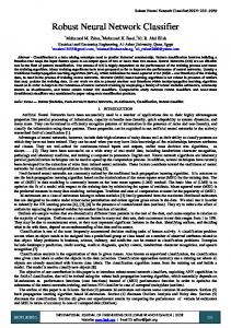
I. INTRODUCTION It is well known that standard feed-forward multi-layer neural networks (NN) trained with gradient descent algorithms such as backpropagation often fail to converge completely in classification problems for a variety of reasons, and much work has been carried out to attempt to improve this situation[1,2]. Failure to converge may be due to an incorrect architecture with too few layers of weights (or too many), or too few hidden neurons. However, in many cases convergence is not achieved for a particular training set because certain neurons saturate before others. In the case of the Multi-Layer Perceptron (MLP) NN with sigmoidal outputs using the logistic function 1/(1+e-x) which has outputs within the range [0,1] or tanh(x) with range [-1,1], the backpropagation algorithm requires multiplication by the derivative of the function in order to make a change in a weight connected to that neuron, and thus carry out gradient descent. Saturation occurs if the output is pushed towards its extremes at some point before convergence is reached, so that the derivative is too small to make further significant weight changes, causing the network to settle in an incorrect local minimum or reach a state of network paralysis (see Figure 1). This saturation may occur for a number of reasons, most of which are easily avoided.
0.7
Neuron Output Activation
The problem of saturation in neural network classification problems is discussed. The listprop algorithm is presented which reduces saturation and dramatically increases the rate of convergence. The technique uses selective application of the backpropagation algorithm, such that training is only carried out for patterns which have not yet been learnt to a desired output activation tolerance. Furthermore, in the output layer, training is only carried out for weights connected to those output neurons in the output vector which are still in error, which further reduces neuron saturation and learning time. Results are presented for a 196-100-46 Multi-Layer Perceptron (MLP) neural network used for text-to-speech conversion, which show that convergence is achieved for up to 99.7% of the training set compared to at best 94.8% for standard backpropagation. Convergence is achieved in 38% of the time taken by the standard algorithm.
Saturation Tolerance (Upper)
Output Activation Tolerance (Upper)
0.9
0.6 0.5 0.4
Upper Saturation Region
Lower Saturation Region
0.3 0.2 0.1 0
Saturation Tolerance (Lower)
Output Activation Tolerance (Lower)
-5 -4.5 -4 -3.5 -3 -2.5 -2 -1.5 -1 -0.5
0
0.5
1
1.5
2
2.5
3
3.5
4
4.5
5
Neuron Sum-of-products
Figure 1 Logistic function 1/(1+e-x ) showing typical saturation limits for a neuron output, and an example output activation tolerance (χ = 0.3) which is below these limits
Five common reasons for saturation occurring are as follows: 1. 2. 3. 4. 5.
Magnitude of the initial weight range is too large Weight quantisation is too coarse The learning rate is too large The training set is not normalised Overtraining
The first of these can be a problem if the initial random weight range i.e. the distribution of initial weights, is not appropriate to the NN architecture. A neuron can saturate immediately if the associated initial random weight vector is unluckily chosen, which becomes more likely for any particular weight range as the number of inputs is increased. Care must thus be taken to reduce the initial weight range as the number of neuron inputs grows. The second reason, which is often relevant in limited precision implementations[3], is avoided by making sure that enough bits are used for the weight changes. The third reason for saturation is avoided by keeping the learning rate as small as possible, which also ensures a better approximation to steepest descent. In this case, however, there is a trade-off with speed of convergence. This problem can be compounded by the use of momentum or some similar second-order technique commonly used in modified forms of backpropagation, which can produce larger weight changes than would be expected from the use of a constant learning rate. Thus it may also be necessary to take care not to make the momentum term too large. The fourth reason is more subtle. In classification problems, if there are more examples of one class than
Proceedings of the Fourth IEEE International Conference on Electronics, Circuits and Systems, Cairo, Egypt, December 15-18 1997, Volume 1, pp 254-258. Copyright © 1997 by the Institute of Electrical and Electronic Engineers Inc.
another, the network becomes biased towards the largest class. In terms of probability this may be desirable, but it may also mean that certain training patterns are simply not learnt if they are in a very small class compared to the others, as the network quickly converges and saturates in favour of the dominant class or classes. This can be avoided in principle by a process of normalisation, which can be carried out by increasing on average the number of times certain patterns are presented per epoch so that all classes are fairly represented. However, this is at the expense of an increase in size of the training set or the number of epochs (e.g. presentations of the entire training set) required for convergence.
M HIDDEN LAYER NEURONS
L INPUTS yi
wji
Θj
xj
yj
N OUTPUT LAYER NEURONS wkj
Θk
yk
xk
Σ
F
Σ
F
Σ
F
Σ
F
Σ
F
Σ
F
Σ
F
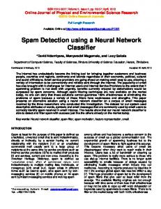
Figure 2 L-M-N multi-layer perceptron neural network architecture
The fifth reason for saturation is the most difficult to prevent and is related to the problem of how to decide when to stop the training procedure. It is desirable to stop training before saturation occurs not least because there is no point training for more epochs than is necessary to separate the classes by a desired margin, even if convergence can be easily achieved, but also to ensure good generalisation since overtraining also has the effect of making the network too finely tuned to idiosyncrasies in the training set. A widely used method of doing this is to stop when all the network outputs have achieved their required target state for all patterns to within a specified tolerance[4]. This is to be preferred over waiting for a minimum total Mean Squared Error to be reached as it is clearer how well the MLP is classifying the input set. For the logistic function an output activation tolerance of χ=0.1 means that an output of 0.1 or smaller is considered to be a logical 0 if that is the desired output, and one of 0.9 or greater is considered to be a logical 1. This works adequately for some training sets like in the EXOR problem where all four patterns are learnt after a similar number of epochs (in fact {(1,1),(0)} is learnt last, but not very long after the others), but quite badly if some classes are easily distinguished when others are separated by complex decision boundaries. In these cases some patterns are always learnt to within the specified tolerance long before others, even if the training set is normalised, resulting in overtraining with the easier ones. One method for avoiding saturation directly, proposed by Fahlman[2], is to bound the weight step away from zero by adding a constant term thus ensuring a minimum weight step. Another method is to use a probabilistic update strategy[5] which is particularly useful in hardware implementations with limited precision. The alternative method of selective backpropagation presented in this paper reduces saturation, and also reduces the number of epochs to convergence and increases the overall number of training patterns which can be learnt over the standard method. It also removes the need for normalisation and improves the speed of convergence in terms of computational steps required.
II. METHOD The typical L-M-N fully interconnected MLP architecture with two layers of weights is shown in Figure 2. The network has L inputs, M hidden layer neurons and N output layer neurons. The output function F is the sigmoidal nonlinearity, or logistic function 1/(1+e-x) which limits the output range between 0 and 1. The inputs and outputs of each layer are denoted by yi for the inputs to the hidden layer (1≤i≤L), yj for the inputs to the output layer (1≤j≤M), and yk for the final outputs (1≤k≤N). The neuron sums-of-products are denoted by xj and xk. The hidden layer weights are denoted by wji, the output layer weights by wkj and the corresponding threshold biases are θj and θk. The usual implementation of the backpropagation algorithm (backprop)[6] consists of two phases; a forward pass (or recall phase) in which an input pattern is presented to the network and the actual outputs are calculated, and a backward pass (or learning phase) in which the errors are calculated and the weights are adjusted. A backward pass is always carried out after each forward pass. The weight changes for each neuron are determined by multiplying the learning rate η (constant for the entire network) by the error term δj or δk (constant for that neuron in any one pass) and the corresponding inputs. When all patterns in the training set have been presented to the network this is recorded as one training epoch. The forward pass is,
L y j = F ∑ w ji y i + θ j , i =1
∀j
(1)
M y k = F ∑ w kj y j + θ k , j =1
∀k
(2)
Proceedings of the Fourth IEEE International Conference on Electronics, Circuits and Systems, Cairo, Egypt, December 15-18 1997, Volume 1, pp 254-258. Copyright © 1997 by the Institute of Electrical and Electronic Engineers Inc.
The number of multiplications per pattern for the sum-ofproducts in the forward pass is MN+LM. Note however that in practice many of the multiplications in the forward pass can be avoided completely for classification problems, since multiplication in equation (1) is either by 0 or 1, so comparison and addition can be used instead. A backward pass is then carried out where these outputs are compared to the desired outputs dk and the delta values for each neuron are calculated,
δ k = y k (1 − y k )( d k − y k ) , ∀k
(3)
weights to all output nodes (with indices 1 to N) in a loop, a list is first made of all n(Γ) outputs still in error (n(Γ)≤N), so that the elements of the list are the indices of these in the order in which they are found. If n(Γ)=0 (i.e. Γ=∅, the empty set), the pattern has been learnt and no backward pass is applied. Otherwise the backward pass is applied to the list of outputs which are in error, as follows,
δ k = y k (1 − y k )( d k − y k ), δ j = y j (1 − y j )∑ w kj δ k ,
(7)
∀j
(8)
k ∈Γ
N
δ j = y j (1 − y j )∑ w kj δ k , ∀j
k ∈Γ
(4)
k =1
This is followed by changing the weights by the following increments,
∆w kj = ηδ k y j , ∀j, k
∆θ k = ηδ k , ∀k
(5)
∆w ji = ηδ j y i , ∀i, j
∆θ j = ηδ j , ∀j
(6)
The total number of multiplications per pattern in the backward pass is 3MN+2(L+1)M+2N, which is much more than in the forward pass, so it is in this phase where much of the time saving can be made. As in equation (1), many of the multiplications in equation (6) can be avoided for binary inputs. In order to check for possible convergence, each of the outputs in the output vector is checked after the forward pass to see whether it has been learnt to the desired output activation tolerance, χ. If this is the case for all outputs in the output vector for every pattern in the training set, the network is said to have learnt to classify the entire training set and training can be terminated. Alternatively training can be carried out for a specified number of epochs. Note that even if some patterns have been learnt to the desired tolerance training is still carried out for these patterns, which can result in saturation due to overtraining. In the proposed alternative algorithm, listprop, a backward pass is carried out for a particular training pattern only if the pattern output has not been learnt to within the tolerance χ. Furthermore if the pattern has not been learnt, the backward pass is only applied to the output neurons in the output vector which have not yet reached the required tolerance, which comprise a set Γ of outputs which are in error i.e. dk-yk≥χ. In this way it is not possible for the output of a neuron which has crossed the tolerance threshold to be changed any further by that pattern unless other patterns in the training set change the weights later on, so as to move the decision boundary to bring it back in error again. Note that simply training the patterns not learnt using the entire output vector is not sufficient to prevent saturation, as individual outputs in the output pattern may become saturated before others. In practice the backward pass is modified so that rather than update the
∆w kj = ηδ k y j , ∀j, k ∈ Γ ∆w ji = ηδ j y i , ∀i, j
∆θ k = ηδ k , k ∈Γ (9) ∆θ j = ηδ j , ∀j
(10)
Thus the number of multiplications for a particular pattern in a particular epoch is reduced to 3Mn(Γ)+2(L+1)M+2n(Γ). As training proceeds, many of the n(Γ) become very small or zero, so that the average training time of the epoch decreases. As the NN converges, some oscillation is to be expected as the remaining patterns compete for the weights which will help them converge. Close to full convergence, the most difficult patterns to learn should gain more and more influence on the weight set which may help a global minimum to be found which is beneficial to all patterns. Clearly this also provides a gain in speed because patterns which have been learnt are taken out of the backward pass, with virtually no overhead as every output has to be checked anyway for possible convergence. This is very advantageous as many networks learn a large proportion of patterns early on in the training procedure, which are usually just overtrained in the conventional implementation.
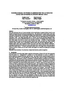
III. EXPERIMENT In order to test the hypothesis, a typical MLP problem was chosen, involving text-to-speech (letter-to-phoneme) conversion, which was a candidate for use as the front end of a speech synthesis system, but was also one with which we had been experiencing non-convergence problems due to saturation. It was also clear that the proposed method would have a most significant effect on the convergence time of a network with a large training set and a large number of outputs. The MLP chosen had a 196-100-46 architecture based on the NETtalk text-to-speech architecture of Sejnowski and Rosenberg[7] but with outputs which selected phonemes in the International Phonetic Alphabet rather than articulatory features. The input data was presented as a window of seven characters which was moved along the running text. The network was trained to pick out the correct phoneme for the central letter of the seven, the other letters being used to
Proceedings of the Fourth IEEE International Conference on Electronics, Circuits and Systems, Cairo, Egypt, December 15-18 1997, Volume 1, pp 254-258. Copyright © 1997 by the Institute of Electrical and Electronic Engineers Inc.
/k / O u tp ut N e uron s
H id de n N e uron s
Inp uts
(
-
a
-
c
a
t
-
)
TEXT
Figure 3 MLP architecture for letter-to-phoneme transcription
Software MLPWIN was written in the C programming language to implement both algorithms in a Microsoft Windows environment, which allowed the required parameters to be set and changed as required. The training set was constructed from a file of text containing 566 of the most commonly written American-English words, obtained from the statistical analysis of Brown’s Corpus by Kucera and Francis[8], and phoneme data derived from a specially designed computer program based on the letterto-phoneme rules of Elovitz et al[9]. The final training set consisted of 2856 letter-to-phoneme mappings, one for each letter of the 566 words placed centrally in the seven character window. Training was carried out for both backprop and listprop using the same initial weight range [-0.01,0.01] and random seed, and learning rates η from 0.4 to 1.9 at intervals of 0.1 in order to make sure the algorithms were compared at their optimum learning rates. A output activation tolerance of χ=0.3 was chosen, which leaves a margin of 1-2χ=0.4 between ‘0’ and ‘1’ at each output. In each case training was stopped after 100 epochs, in order to compare the percentage of patterns learnt and the total time taken for the training. After training, generalisation ability was tested by recall of a further 2956 patterns, using the next 465 most common words from Brown’s Corpus.
The most significant improvement is in the training time for listprop which is only 38% of the time required for backprop. Generalisation capability is also better with listprop, although this is probably accounted for by the improved convergence for the training set. Evidence of oscillation is apparent for listprop at all learning rates. However this effect is small, and percentage convergence at the higher learning rates is not much different, these being 99.6% for η=1.4 and 99.3% for η=1.9. This should be compared to figures of 94.5% for η=1.4 and 94.5% for η=1.9 for backprop, suggesting saturation had occurred. Indeed, by examining the network outputs it was seen that some of the these were very close to 0 or 1 for many of the patterns in the training set, and training for a further 100 epochs did not improve the result. Examination of the graphs shows that the curves have a smoother ‘knee’ for the listprop training in Figure 5 than the ones for backprop in Figure 4. The difference is especially noticeable at higher learning rates. This indicates that the new algorithm has overcome the problem of early overtraining.
100% 90% 80% Patterns Learnt
PHO N EM E
results from the generalisation testing. It can be seen that the listprop algorithm is superior in respect of the number of patterns learnt to the required convergence criteria with a best percentage convergence of 99.7% for η=0.9 compared to a best of 94.8% for backprop, also for η=0.9.
Learning Rate=0.4
70% 60% 50% 40% 30%
Learning Rate=0.9 Learning Rate=1.4
20% 10% 0%
Learning Rate=1.9
0
10
20
30
40
50
60
70
80
90
100
Epochs
Figure 4 Graph for backprop training with various learning rates
100% 90% 80% Patterns Learnt
provide a context for the transcription. Figure 3 shows a schematic of the architecture. The inputs consist of 7 groups of 28 bits, of which one bit in each group is a ‘1’ and the rest ‘0’. The ‘1’ represents the selection from a set of 28 possible characters, the 26 letters of the alphabet plus 2 for punctuation. Hence, only seven of the inputs are ‘1’ for any input pattern. A hidden layer of 100 neurons has been found necessary to be able to capture the regularities in English text. The phoneme classification was made by selection of one of a representative set of 46 phonemes.
70% Learning Rate=0.4
60% 50%
Learning Rate=0.9
40% Learning Rate=1.4
30% 20%
Learning Rate=1.9
10% 0% 0
10
20
30
40
50
60
70
80
90
100
Epochs
IV. RESULTS The results of the training using the MLPWIN software executed on an IBM-compatible PC with an Intel 486DX 66MHz processor are shown by the graphs in Figures 4 and 5 for backprop and listprop respectively, and by the timings table in Figure 6. The table in Figure 7 shows the
Figure 5 Graph for listprop training with various learning rates
Proceedings of the Fourth IEEE International Conference on Electronics, Circuits and Systems, Cairo, Egypt, December 15-18 1997, Volume 1, pp 254-258. Copyright © 1997 by the Institute of Electrical and Electronic Engineers Inc.
VI. REFERENCES Learning Rate
0.4
0.9
1.4
1.9
Total training time for 100 epochs (seconds) backprop 15073 15527 15063 15526 listprop 6142 5877 6093 5812 Figure 6 Comparison of time taken for training using backprop and listprop algorithms
Learning Rate
0.4
0.9
1.4
1.9
Percentage of non-training patterns correctly classified backprop 85.9 86.8 87.7 87.1 listprop 88.6 88.8 87.3 87.6 Figure 7 Comparison of percentage of patterns correctly classified in generalisation testing of backprop and listprop trained networks
V. CONCLUSIONS The results show that by using selective backpropagation (listprop) a neural network classifier can learn faster, and with a greater percentage of training patterns classified correctly. Generalisation performance was also improved in line with the improvement in convergence, suggesting that classification ability is not affected by the smaller margin (1-2χ) which results from training to a specified output activation tolerance. The case study is typical of the type of large network problem which would benefit greatly from a reduction in training time, which in the text-tospeech example was 38% of the time required to train with the standard algorithm. In addition the proposed alternative algorithm does not appear to be sensitive to the learning rate, and oscillation was not found to be a problem. The techniques used to improve the standard backpropagation algorithm may find further use in the improvement of existing modified forms of the backpropagation algorithm for classification problems, and in hardware implementations with limited precision.
[1] LOONEY C.G. : “Stabilisation and Speedup of Convergence in Training Feedforward Neural Networks”, Neurocomputing, 10 ,1996, pp7-31. [2] FAHLMAN S.E. : “An Empirical Study of Learning Speed in Back-Propagation Networks”, Technical Report CMU-CS-88-162, Carnegie Mellon University, Pittsburgh PA, June 1988. [3] HOLLIS P.W., HARPER J.S. and PAULOS J.J. : “The Effects of Precision Constraints in a Backpropagation Learning Network”, Neural Computation 2, pp363-373, 1990 [4] RUMELHART D.E., and McCLELLAND (Eds.) : “Parallel Distributed Processing : Explora-tions in the Microstructure of Cognition, Vol I : Foundations” (MIT Press 1986). [5] HOEHFELD M. and FAHLMAN S.E. : “Probabilistic Rounding in Neural Network Learning with Limited Precision”, Proc. IEEE/ITG/IFIP 2nd Int. Workshop on Microelectronics for Neural Networks, Munich, pp1-8, Oct 1991. [6] RUMELHART D.E., HINTON G.E. and WILLIAMS M.J. : “Learning Internal Representations by Backpropagation of Errors”, Nature 323, pp533-536, 1986. [7] SEJNOWSKI T.J., and ROSENBERG C.R. : “Parallel Networks that Learn to Pronounce English Text”, Complex Systems 1, pp145-168, 1987. [8] KUCERA H. and FRANCIS W.N. : “Computational Analysis of Present Day American English”, (Brown University Press, Providence RI, 1970). [9] ELOVITZ H.S., JOHNSON R., McHUGH A., and SHORE J.E. : “Letter-to-Sound Rules for Automatic Translation of English Text to Phonetics”, IEEE Trans. Acoustics, Speech, and Signal Processing, 24(6), 1976.