Hindawi Publishing Corporation Mathematical Problems in Engineering Volume 2015, Article ID 581909, 12 pages http://dx.doi.org/10.1155/2015/581909
Research Article A Fault-Tolerant Filtering Algorithm for SINS/DVL/MCP Integrated Navigation System Xiaosu Xu,1 Peijuan Li,2 and Jian-juan Liu3 1
Key Laboratory of Micro-Inertial Instrument and Advanced Navigation Technology, Ministry of Education, School of Instrument Science & Engineering, Southeast University, Nanjing 210096, China 2 Industrial Center, Nanjing Institute of Technology, Nanjing 211167, China 3 Henan University of Technology, Zhengzhou 450007, China Correspondence should be addressed to Xiaosu Xu;
[email protected] Received 3 July 2014; Revised 13 April 2015; Accepted 15 April 2015 Academic Editor: Filippo Ubertini Copyright © 2015 Xiaosu Xu et al. This is an open access article distributed under the Creative Commons Attribution License, which permits unrestricted use, distribution, and reproduction in any medium, provided the original work is properly cited. The Kalman filter (KF), which recursively generates a relatively optimal estimate of underlying system state based upon a series of observed measurements, has been widely used in integrated navigation system. Due to its dependence on the accuracy of system model and reliability of observation data, the precision of KF will degrade or even diverge, when using inaccurate model or trustless data set. In this paper, a fault-tolerant adaptive Kalman filter (FTAKF) algorithm for the integrated navigation system composed of a strapdown inertial navigation system (SINS), a Doppler velocity log (DVL), and a magnetic compass (MCP) is proposed. The evolutionary artificial neural networks (EANN) are used in self-learning and training of the intelligent data fusion algorithm. The proposed algorithm can significantly outperform the traditional KF in providing estimation continuously with higher accuracy and smoothing the KF outputs when observation data are inaccurate or unavailable for a short period. The experiments of the prototype verify the effectiveness of the proposed method.
1. Introduction Integration technology has become one of the key issues in navigation because of its capability of overcoming the drawbacks of single strapdown inertial navigation system (SINS), such as error accumulation and error swing over a period of time. The most commonly used navigation systems are radio and satellite based system, including global positioning system (GPS) [1] and Doppler velocity log (DVL) [2, 3]; their performance is fundamentally limited by propagation of signals [4, 5]. The integrated navigation system proposed in this work is an economic navigating algorithm of high precision, in which the SINS is integrated with a DVL and a magnetic compass (MCP). The Kalman filter (KF) is an effective optimal estimation algorithm and has been widely used in integrated navigation system since 1970s [6–9]. On one hand, in order to achieve a better performance with a KF, an accurate system model
and reliable observation data are indispensable. Moreover, the KF fails to estimate the state vector exactly when the observations noise increases [10–12]. However, in real engineering applications, it is usually difficult to satisfy the above conditions. For example, undersea DVL’s output will be interfered or broken owing to the cliffy sea bottom and other vessel reflections [13, 14]. In order to solve this problem, the following method is often adopted: if the observation data from DVL or MCP are temporarily inaccurate or inaccessible, the integrated navigation system can be compromised to work under pure inertial mode. But, it is evident that the measuring accuracy will deteriorate remarkably and the system error will accumulate or swing over time in pure inertial mode. After the system returns to the integration mode when the observation data are recovered, the position error will definitely not be compensated although the errors of velocities and attitude angles can be reduced. Therefore, a fault-tolerant filtering algorithm that can maintain
2
Mathematical Problems in Engineering
the accuracy of an integrated navigation system through inexact or unavailable observation data is important and urgent [15–17]. Evolutionary programming, put forward by Fogel [18], is essential for random searching in that it boosts the survival of the fittest and organic evolution mechanism and searches for the optimal point in feasible space via population search strategy [19, 20]. Moreover, the artificial neural network (ANN), optimized by evolutionary programming, not only overcomes the obstacle of conventional ANN which may easily plunge into local minimum and requires long training time, but also avoids the problem in genetic algorithms caused by binary-coded and cross operation. Thanks to its superiorities, ANN has been applied in many fields such as financial forecasting [21], breast cancer diagnosis [22], and electricity supply industry [23], and so forth [24]. In this paper, a fault-tolerant integrated navigation system with an adaptive Kalman filter (AKF) based on evolutionary artificial neural networks (EANN) is proposed, in which the EANN is used in self-learning and training of the intelligent data fusion algorithm. The proposed fault-tolerant adaptive Kalman filter (FTAKF) algorithm is able to maintain a smooth output under the condition when observation data are inaccurate or unavailable. The prototype experiment indicates that the algorithm can efficiently outperform the traditional KF with a higher accuracy when observation data are inaccurate or unavailable. This paper is organized as follows. In Section 2, the inertial error model is introduced and a corresponding mathematical model in state and measurement space is described. In Section 3, we propose the AKF algorithm and compare its characteristics and properties with those of traditional KF algorithm. A fast ANN based on evolutionary programming is proposed in Section 4. In Sections 5 and 6, applications of algorithm in SINS/DVL/MCP are presented and several tests are conducted to evaluate the performance of the intelligent navigation system with FTAKF. Conclusions are made in Section 7.
2. Mathematical Model for Filter
C𝑛𝑏
𝑐𝛾 𝑐𝜓 + 𝑠𝛾 𝑠𝜓 𝑠𝜃 𝑠𝜓 𝑐𝜃 𝑠𝛾 𝑐𝜓 − 𝑐𝛾 𝑠𝜓 𝑠𝜃 ] [ [ = [−𝑐𝛾 𝑠𝜓 + 𝑠𝛾 𝑐𝜓 𝑠𝜃 𝑐𝜓 𝑐𝜃 −𝑠𝛾 𝑠𝜓 − 𝑐𝛾 𝑐𝜓 𝑠𝜃 ] ]. −𝑠𝛾 𝑐𝜃 𝑠𝜃 𝑐𝛾 𝑐𝜃 ] [
(1) Inertial Error Model. Here we define the navigation coordinates frame as an east-north-vertical (ENV) geography coordinates frame. The attitude angle, velocity, and position errors are given in the following. Attitude angle error is determined by (1)
where 𝜙𝑛 = [𝜙𝐸 , 𝜙𝑁, 𝜙𝑈]Τ is the orientation error vector of the calculated platform represented in the navigation coordinates frame, 𝜔𝑛𝑖𝑒 = [0, 𝜔𝑖𝑒 cos 𝐿, 𝜔𝑖𝑒 sin 𝐿]Τ represents the rotation projection of the earth onto the ENV axes with 𝜔𝑖𝑒 = 7.292115×10⁻⁵ rad/s to be the angular velocity of the rotation
(2)
Velocity error is defined as 𝛿V̇ 𝑛 = f 𝑛 × 𝜙𝑛 − (2𝛿𝜔𝑛𝑖𝑒 + 𝛿𝜔𝑛𝑒𝑛 ) × V𝑛 − (2𝜔𝑛𝑖𝑒 + 𝜔𝑛𝑒𝑛 ) × 𝛿V𝑛 + C𝑛𝑏 ∇𝑏 ,
(3)
where 𝛿V𝑛 = [𝛿𝑉𝐸 , 𝛿𝑉𝑁, 𝛿𝑉𝑈]Τ viewed as the linear velocity error vector is determined by the specific force vector f 𝑛 =[𝑓𝐸 , 𝑓𝑁, 𝑓𝑈]Τ and the bias vector ∇𝑏 = [∇𝑥 , ∇𝑦 , ∇𝑧 ] of accelerometer in the body coordinates frame, along with 𝛿𝜔𝑛𝑖𝑒 and 𝛿𝜔𝑛𝑒𝑛 that represent the slow variations of 𝜔𝑛𝑖𝑒 and 𝜔𝑛𝑒𝑛 , 𝑏 respectively. Here, ∇̇ = 0. Position error is given by 𝛿𝑉𝑁 𝑉𝑁 𝛿𝐿̇ = 𝛿ℎ, − 𝑅𝑛 + ℎ (𝑅𝑛 + ℎ)2 𝛿𝑉𝐸 𝑉𝐸 𝛿𝜆̇ = sec𝐿 + sec 𝐿tan 𝐿𝛿𝐿 Re + ℎ Re + ℎ −
2.1. Error Model of Integrated Navigation System
𝑛 𝜙̇ = 𝛿𝜔𝑛𝑖𝑒 + 𝛿𝜔𝑛𝑒𝑛 − (𝜔𝑛𝑖𝑒 + 𝜔𝑛𝑒𝑛 ) × 𝜙𝑛 + C𝑛𝑏 𝜀𝑏 ,
of the earth, and 𝜔𝑛𝑒𝑛 = [−𝑉𝑁/(𝑅𝑛 + ℎ), 𝑉𝐸 /(𝑅𝑒 + ℎ), (𝑉𝐸 /(𝑅𝑒 + ℎ)) tan 𝐿]Τ denotes the angular velocity of the rotation of a navigation coordinates frame relative to the earth with 𝑉𝐸 , 𝑉𝑁, and 𝑉𝑈 that represent the linear velocities, 𝜆, 𝐿, and ℎ that represent the position coordinates (longitude latitude and height, resp.), and 𝑅𝑛 , 𝑅𝑒 that represent the radii of the curvatures along the meridian and parallel, respectively (Table 2). Moreover, 𝜀𝑏 = [𝜀𝑥 , 𝜀𝑦 , 𝜀𝑧 ] is the gyro-drifts in the body coordinates frame with 𝜀̇𝑏 = 0. The last term C𝑛𝑏 represents the attitude matrix, which can be expressed by the attitude angles 𝜓, 𝛾, and 𝜃. Given the definition [𝑠𝜓 , 𝑐𝜓 , 𝑠𝛾 , 𝑐𝛾 , 𝑠𝜃 , 𝑐𝜃 ]Τ = [sin 𝜓, cos 𝜓, sin 𝛾, cos 𝛾, sin 𝜃, cos 𝜃]Τ , C𝑛𝑏 can be written as
𝑉𝐸
(Re + ℎ)2
(4)
sec 𝐿𝛿ℎ,
𝛿ℎ̇ = 𝛿𝑉𝑈, where 𝛿𝜆, 𝛿𝐿, and 𝛿ℎ represent the position errors. (2) DVL Error Model. The velocity of DVL in the body coor̃𝑑 can be described as follows: dinates frame V ̃𝑑 = (I + 𝛿K) V𝑑 + 𝛿V𝑑 . V
(5)
Here, 𝛿K = [𝛿𝐾𝑑𝑥 , 𝛿𝐾𝑑𝑦 , 𝛿𝐾𝑑𝑧 ]Τ is the scale factor error assumed to be random constant and 𝛿K̇ = 0 and 𝛿V𝑑 = [𝛿𝑉𝑑𝑥 , 𝛿𝑉𝑑𝑦 , 𝛿𝑉𝑑𝑧 ]Τ represents the linear velocity errors of
Mathematical Problems in Engineering
3
DVL, which can be characterized by first-order Markov process as ̇ =− 𝛿𝑉𝑑𝑥
𝛿C𝑛𝑏 = (I − C𝑝𝑛 ) C𝑛𝑏 ,
1 𝛿𝑉 + 𝑤𝑑𝑥 , 𝜏𝑑𝑥 𝑑𝑥
̇ = − 1 𝛿𝑉𝑑𝑦 + 𝑤𝑑𝑦 , 𝛿𝑉𝑑𝑦 𝜏𝑑𝑦
(6)
where 𝜏𝑑 = [𝜏𝑑𝑥 , 𝜏𝑑𝑦 , 𝜏𝑑𝑧 ]Τ is the time correlation coefficient of this Markov process and w𝑑 = [𝑤𝑑𝑥 , 𝑤𝑑𝑦 , 𝑤𝑑𝑧 ]Τ is the input noise of DVL. (3) MCP Error Model. Heading attitude angle error of MCP 𝛿𝜓𝑚 can be represented as first-order Markov process with (7)
where 𝜏𝑚 is the time correlation coefficient and 𝑤𝑚 is the input noise of MCP.
where 𝑝 is the calculating navigation coordinate frame. Substituting (12) into (11), it yields
(8)
where matrices F and Γ can be established from the above error model and W is the input (system) noise:
̃𝑛 − V ̃𝑛 + 𝜂 ΔV𝑛 = V 𝑑 𝑑 = V𝑛 + 𝛿V𝑛 − V𝑛𝑑 − (I − C𝑝𝑛 ) C𝑛𝑏 C𝑏𝑑 V𝑑 + 𝜂𝑑
where the measurement velocity vector ΔV𝑛 = [Δ𝑉𝐸 , Δ𝑉𝑁, Δ𝑉𝑈] and 𝛿V𝑛𝑑 = (I − C𝑝𝑛 )C𝑛𝑏 C𝑏𝑑 V𝑑 can be calculated from 𝛿𝑉𝑑𝐸 = 𝜙𝑈𝑉𝑁 − 𝜙𝑁𝑉𝑈 + C𝑛𝑏 (1, 1) 𝛿𝑉𝑑𝑥 + C𝑛𝑏 (1, 2) 𝛿𝑉𝑑𝑦 + C𝑛𝑏 (1, 3) 𝛿𝑉𝑑𝑧 + C𝑛𝑏 (1, 1) 𝑉𝐸 𝛿𝐾𝑑𝑥 + C𝑛𝑏 (1, 2) 𝑉𝑁𝛿𝐾𝑑𝑦 + C𝑛𝑏 (1, 3) 𝑉𝑈𝛿𝐾𝑑𝑧 , 𝛿𝑉𝑑𝑁 = 𝜙𝐸 𝑉𝑈 − 𝜙𝑈𝑉𝐸 + C𝑛𝑏 (2, 1) 𝛿𝑉𝑑𝑥 + C𝑛𝑏 (2, 2) 𝛿𝑉𝑑𝑦 + C𝑛𝑏 (2, 3) 𝛿𝑉𝑑𝑧 + C𝑛𝑏 (2, 1) 𝑉𝐸 𝛿𝐾𝑑𝑥 + C𝑛𝑏 (2, 2) 𝑉𝑁𝛿𝐾𝑑𝑦
(9)
𝛿𝑉𝑑𝑈 = 𝜙𝑁𝑉𝐸 − 𝜙𝐸 𝑉𝑁 + C𝑛𝑏 (3, 1) 𝛿𝑉𝑑𝑥 + C𝑛𝑏 (3, 2) 𝛿𝑉𝑑𝑦 + C𝑛𝑏 (3, 3) 𝛿𝑉𝑑𝑧 + C𝑛𝑏 (3, 1) 𝑉𝐸 𝛿𝐾𝑑𝑥 + C𝑛𝑏 (3, 2) 𝑉𝑁𝛿𝐾𝑑𝑦
X = [𝛿𝑉𝐸 , 𝛿𝑉𝑁, 𝛿𝑉𝑈, 𝜙𝐸 , 𝜙𝑁, 𝜙𝑈, 𝛿𝐿, 𝛿𝜆, 𝛿ℎ, ∇𝑥 , ∇𝑦 ,
Similarly, after differentiating the heading angle of SINS and MCP, the measurement model is given as
2.3. Measurement Space. Supposing that the error of the velocity of DVL in the navigation coordinates frame V𝑛𝑑 is ̃𝑛 can mainly caused by platform misalignment, the error of V 𝑑 be described as
where C𝑏𝑑
+ C𝑛𝑏 (3, 3) 𝑉𝑈𝛿𝐾𝑑𝑧 .
(10)
𝛿𝜓𝑚 ] .
̃𝑛 V 𝑑
(15)
+ C𝑛𝑏 (2, 3) 𝑉𝑈𝛿𝐾𝑑𝑧 ,
where 𝑤𝑔𝑥 , 𝑤𝑔𝑦 , and 𝑤𝑔𝑧 are the white noise of the gyros and 𝑤𝑎𝑥 , 𝑤𝑎𝑦 , and 𝑤𝑎𝑧 are the white noise of the accelerometers. The state vector X of the integrated navigation system is defined as
∇𝑧 , 𝜀𝑥 , 𝜀𝑦 , 𝜀𝑧 , 𝛿𝑉𝑑𝑥 , 𝛿𝑉𝑑𝑦 , 𝛿𝑉𝑑𝑧 , 𝛿𝐾𝑑𝑥 , 𝛿𝐾𝑑𝑦 , 𝛿𝐾𝑑𝑧 ,
(14)
= 𝛿V𝑛 − (I − C𝑝𝑛 ) C𝑛𝑏 C𝑏𝑑 V𝑑 + 𝜂𝑑 ,
W = [ 𝑤𝑔𝑥 , 𝑤𝑔𝑦 , 𝑤𝑔𝑧 , 𝑤𝑎𝑥 , 𝑤𝑎𝑦 , 𝑤𝑎𝑧 , 𝑤𝑑𝑥 , 𝑤𝑑𝑦 , 𝑤𝑑𝑧 , 𝑤𝑚 ] ,
(13)
After differentiating the velocity of SINS and DVL, the measurement model can be written as
2.2. State Space. The error models given in (1), (3)-(4), and (6)-(7) have a standard form given by Ẋ = F ⋅ X + Γ ⋅ W,
(12)
̃𝑛 = V𝑛 + (I − C𝑝 ) C𝑛 C𝑏 V𝑑 . V 𝑑 𝑑 𝑛 𝑏 𝑑
̇ = − 1 𝛿𝑉𝑑𝑧 + 𝑤𝑑𝑧 , 𝛿𝑉𝑑𝑧 𝜏𝑑𝑧
1 𝛿𝜓̇𝑚 = − 𝛿𝜓𝑚 + 𝑤𝑚 , 𝜏𝑚
frame. The perturbation of the attitude matrix 𝛿C𝑛𝑏 is defined as
=
V𝑛𝑑
+ 𝛿V𝑛𝑑
=
V𝑛𝑑
+ 𝛿C𝑛𝑏 C𝑏𝑑 V𝑑 ,
=
C𝑛𝑏 C𝑏𝑑 V𝑑
+ 𝛿C𝑛𝑏 C𝑏𝑑 V𝑑
(11)
is a constant matrix which translates the velocity of DVL V𝑑 from the instrumental frame to the body coordinates
Δ𝜓 = 𝜓̃ − 𝜓̃𝑚 + 𝜂𝑚 = 𝜓 + 𝛿𝜓 − 𝜓𝑚 − 𝛿𝜓𝑚 + 𝜂𝑚 = 𝛿𝜓 − 𝛿𝜓𝑚 + 𝜂𝑚 ,
(16)
where 𝛿𝜓 = −
−
C𝑛𝑏 (1, 2) ⋅ C𝑛𝑏 (3, 2) 2
[C𝑛𝑏 (1, 2)] + [C𝑛𝑏 (2, 2)] C𝑛𝑏 (2, 2) ⋅ C𝑛𝑏 (3, 2) 2
2
𝜙𝐸 (17)
2
[C𝑛𝑏 (1, 2)] + [C𝑛𝑏 (2, 2)]
𝜙𝑁 + 𝜙𝑈.
4
Mathematical Problems in Engineering
Based on the previous analysis, the measurement model is defined as
DVL
Z𝑘 = H𝑘 X𝑘 + 𝜂𝑘 ,
(18)
where Z = [Δ𝑉𝐸 , Δ𝑉𝑁, Δ𝑉𝑈, Δ𝜓]Τ is the observation vector, H𝑘 is the observation matrix at the moment of 𝑘 which can be established from (15) and (17), and vector 𝜂𝑘 represents the Gaussian measurement noise with zero mean value and covariance matrix R.
Velocity
MCP Heading angle Solution
Velocity SINS
Attitude
AKF Position
Error compensation
3. AKF Algorithm to Integrated Navigation System
Figure 1: AKF scheme of SINS/DVL/MCP.
Given the differential equations, we can have a continuous state transition matrix F for error states. The continuous transition matrix can be discretized for KF application by using the first-order Taylor series approximation. The corresponding discrete transition matrix can be computed as Φ = I + FΔ𝑇,
VE
ΔVE VN
(19)
𝛾
where Δ𝑇 is chosen as 0.01 s. Thus, the state equations and observation equation can be written as
𝜃
X𝑘 = Φ𝑘,𝑘−1 X𝑘−1 + Γ𝑘−1 W𝑘−1 ,
𝜓
(20)
Z𝑘 = H𝑘 X𝑘 + 𝜂𝑘 ,
.. .
ΔVN .. .
Δ𝜓
Input layer
where X𝑘 is the 22-dimensional state vector at the moment of 𝑘, Z𝑘 is the 4-dimensional observation vector at the moment of 𝑘, Φ𝑘,𝑘−1 is state-transfer-matrix from sample time 𝑘 − 1 to 𝑘, Γ𝑘−1 is the system noise matrix at the moment of 𝑘 − 1, and W𝑘−1 is system noise. Here, {W𝑘 } and {𝜂𝑘 } are uncorrelated white noise sequences with zero mean. So we can have 𝐸{W𝑘 W𝑗 } = Q𝑘 𝛿𝑘𝑗 and 𝐸{𝜂𝑘 𝜂𝑗 } = R𝑘 𝛿𝑘𝑗 . Q𝑘 is the variance matrix of system noise and R𝑘 is the variance matrix of observation noise. The equations of AKF based on the new information sequence are written as ̂ ̂𝑘/𝑘−1 = 𝜙 X 𝑘,𝑘−1 X𝑘−1 , ̂𝑘/𝑘−1 , V𝑘 = Z𝑘 − H𝑘 X P𝑘/𝑘−1 = K𝑘−1 V𝑘 VT𝑘 KT𝑘−1 + P𝑘−1 , −1
K𝑘 = P𝑘/𝑘−1 HT𝑘 (H𝑘 P𝑘/𝑘−1 HT𝑘 + R𝑘 ) ,
(21)
̂𝑘/𝑘−1 + K𝑘 V𝑘 , ̂𝑘 = X X P𝑘 = (I − K𝑘 H𝑘 ) P𝑘/𝑘−1 . Compared with traditional KF equations, there are two differences. Firstly, Q𝑘 does not appear in above filter equations. That is to say, the statistical properties of the system noise are not needed in AKF, which is a highlight of this algorithm. Secondly, the initial value K0 is needed, and it can be obtained by applying the traditional KF in the first loop. The AKF scheme of the integrated navigation system is shown in Figure 1.
Output layer
Figure 2: Artificial neural networks model.
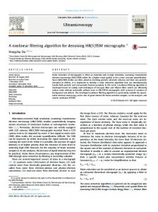
4. Evolutionary Artificial Neural Networks In recent years, ANN has been widely used in various fields, especially the backpropagation (BP) training [25]. However, drawbacks like poor convergence and failure in obtaining the global optimum are the bottleneck in the practical applications [26]. Articles [27–29] use genetic algorithms to optimize the parameters of neural networks. But there exist some imperfections. In this work, evolutionary programming is used to optimize the structure and connection weights in neural networks. 4.1. Artificial Neural Networks Model. ANN theory has proved that three-layer feedforward networks containing only one hidden layer can be a nonlinear mapping of any system with any precision [30]. According to this, the ANN model used in this paper consists of an input layer, a hidden layer, and an output layer. The network structure shown in Figure 2 treats the output navigation parameters of SINS as the input of the networks and the measurement errors as the output of the networks. Considering the limitation of underwater experimental environment, tests are conducted on a land vehicle, and the experimental area is flat and the speed of the vertical direction 𝑉𝑈 can be regarded as zero. Hence, there are 5 nodes in input layer while there are 3 in output layer.
Mathematical Problems in Engineering
5
Based on the assumption that the number of hidden layer )T , and nodes is 𝑚, we have x ∈ R𝑚 , x = (𝑥0 , 𝑥1 , . . . , 𝑥𝑚−1 the connection weights between input and hidden layers are 𝜛𝑖𝑗 (𝑖 = 0, 1, . . . , 4; 𝑗 = 0, 1, . . . , 𝑚 − 1), with thresholds to be Θ𝑗 . The connection weights between output and hidden layers are represented as 𝜛𝑗𝑘 (𝑘 = 0, 1, 2), with thresholds to be Θ𝑘 . Then the output of each layer can be written as 4
𝑥𝑗 = 𝑓1 (∑𝜛𝑖𝑗 𝑥𝑖 − Θ𝑗 ) , 𝑖=0
𝑚−1
(22)
𝑦𝑘 = 𝑓2 ( ∑ 𝜛𝑗𝑘 𝑥𝑗 − Θ𝑘 ) , 𝑗=0
where 𝑓1 and 𝑓2 are transfer functions. In order to study the nonlinear properties of biological neurons, usually 𝑓1 is chosen as a sigmoid function 𝑓1 (𝑥) = 1/(1 + 𝑒−𝑥 ) and 𝑓2 is chosen as a linear function 𝑓2 (𝑥) = 𝑥. During optimizing, the threshold value is treated as import power with value of −1. 4.2. Artificial Neural Networks Optimized by Evolutionary Programming. Darwin’s evolutionary programming is a new search algorithm which is largely dependent on the mutation operator, while the genetic algorithms rely greatly on the crossover operator. When using the evolutionary programming as an optimization algorithm, users need not to be constrained to a particular code structure (representation) or a mutation strategy (evolution operator). Therefore, the flexibility and convenience of evolutionary programming make it surpass the conventional genetic algorithm. The steps for ANN optimization with the network structure and parameters using evolutionary programming are described as follows. (1) Initialization. Here the population of neural networks is set by an initial quantity and the number of hidden layer neurons and the connection weights are initialized randomly within a certain range. Population can be expressed as P = {𝑋1 , 𝑋2 , . . . , 𝑋2𝑁}, where 𝑋𝑖 (𝑖 = 1, 2, . . . , 2𝑁) is the weight distribution of the network and defined as 𝑋𝑖 = [𝑊1 , 𝑊2 , . . . , 𝑊𝑀] with 𝑊𝑘 (𝑘 = 1, 2, . . . , 𝑀) to be the weight between every two connecting nodes of the network. (2) Performance Calculation and Categorization. The training procedure of neural networks uses the overall mean square deviation as a metric. Training will be terminated if the networks’ overall mean square deviation is less than a preset value. Here, the set error is defined as the individual survival environment, which is the goal of every individual evolutionary. For each individual, the fitness function is defined as 𝑓=
1 , 1+𝐸 𝑝
3 1 2 𝐸 = ∑ ∑ (𝑑𝑘 − 𝑜𝑘 ) , 2 𝑙=1 𝑘=1
(23)
where 𝑝 is the number of the imported samples and 𝑑𝑘 and 𝑜𝑘 are the desired and actual outputs of the node 𝑘 of the output layer. Each individual is sorted in a descending order according to fitness. (3) Termination Condition Check. When the best individual meets the requirement or number of loops exceeds the limitation of evolutionary generation, turn to Step (5); otherwise continue. (4) New Population Generation. Firstly, 𝑛 individuals in the current generation are picked as part of the next generation, while removing the rest. Secondly, 𝑛 new individuals are generated from individuals selected by mutation. These 2𝑛 individuals gather to form the new population. Here Gaussian variation is used as the mutation operator. Moreover, according to the characteristics of BP neural networks, the actual error of network is introduced as the enlightening knowledge in the formula; namely, 𝑊𝑘 (𝑡 + 1) = 𝑊𝑘 (𝑡) + Δ𝑊𝑘 , Δ𝑊𝑘 = 𝐿√
1 𝑁 (0, 1) , 𝐹𝑋𝑖
𝐿 = 𝐶 exp
(24)
𝑛 , 𝑛max
where 𝑊𝑘 (𝑡 + 1) and 𝑊𝑘 (𝑡) are the weights of the (𝑡 + 1)th generation and (𝑡)th generation, respectively, with subscript to be 𝑘 = 1, 2, . . . , 𝑀, 𝑁(0, 1) represents a standard normal distribution, 𝐿 and 𝐶 are definition coefficients, 𝑛max is the maximum training cycles of the network, and 𝑛 is the number of the individual survival generations. When the new population is generated, jump to Step (2). (5) Termination Cycle. Terminate the evolution procedure and then train the optimal neural networks using BP algorithm until all requirements are met.
5. Applications of Algorithm in SINS/DVL/MCP On account of the previous algorithm, the FTAKF method based on EANN technology can be applied to the SINS/DVL/ MCP integrated system. The integrated navigation system with an EANN based AKF is shown in Figure 3. When the observation data are diagnosed as available and reliable, EANN works at training state and uses SINS velocity and attitude information as input while the measurement errors are treated as the desired output. In this case switch 1 is connected and switch 2 is off. When the observation data is unavailable or unreliable, EANN works at forecasting state, with switch 1 to be off and switch 2 to be connected.
6
Mathematical Problems in Engineering 𝜒2 fault detection module Observation data
−
S1
Adaptive Kalman filter S2
Network output
Evolutionary neural networks
Output correction
Network input SINS
−
Feedback correction
Figure 3: Integrated navigation system blocks diagram based on evolutionary neural networks.
Here, we use 𝜒2 detecting method to judge whether the observation data is available [31]. When no fault occurs, the residual of filter belongs to white noise, where V𝑘 ∼ 𝑁 (0, A𝑘 ) .
(25)
The mean of V𝑘 is 0 and its variance is A𝑘 = H𝑘 P𝑘/𝑘−1 HT𝑘 + R𝑘 .
(27)
2
where 𝛾𝑘 obeys the 𝜒 distribution and its degree of freedom is 𝑚; that is, 𝛾𝑘 ∼ 𝜒2 (𝑚), and 𝑚 is the dimension of observations vector Z𝑘 . Then, the detection criteria are as follows: if 𝛾𝑘 ≥ 𝑇𝐷, observation data are unavailable, if 𝛾𝑘 < 𝑇𝐷, observation data are available,
Terms Accelerometer biases (g) Accelerometer nonlinearity (% FS) Accelerometer resolution (mg) Gyro biases (∘ /hr) Gyro nonlinearity (% FS) Random walk (∘ /hr1/2 )
Parameters