COMPUTER-AIDED DESIGN Computer-Aided Design 33 (2001) 653±669
www.elsevier.com/locate/cad
A feature-based inspection and machining system T.R. Kramer*, H. Huang, E. Messina, F.M. Proctor, H. Scott Intelligent Systems Division, MS8230, National Institute of Standards and Technology, Gaithersburg, MD 20899, USA Received 1 November 1999; revised 16 September 2000; accepted 15 October 2000
Abstract This paper 1 describes an architecture for a system for machining and inspecting mechanical piece parts and an implementation of it called the Feature-Based Inspection and Control System (FBICS). In FBICS, the controller of a machining center or coordinate measuring machine uses a standard feature-based description of the shape of the object to be made as a principal input for machining and/or inspection. FBICS is a hierarchical control system and performs automated hierarchical process planning. FBICS serves: (1) to demonstrate feature-based inspection and control in an open-architecture control system; (2) as a testbed for solving problems in feature-based manufacturing; and (3) to test the usability of STEP methods and models. q 2001 Published by Elsevier Science Ltd. Keywords: Inspection; NC milling; Process planning; Form features
1. Introduction This paper describes an architecture for a system for machining and inspecting mechanical piece parts, and an implementation of it developed at the National Institute of Standards and Technology (NIST). The system is called the Feature-Based Inspection and Control System (FBICS). This paper covers all aspects of FBICS. Other papers and reports on FBICS include: a much deeper overall description of FBICS [1]; a brief overview of FBICS [2]; a view of FBICS as used in an inspection workstation [3]; and a discussion of process planning in FBICS [4]. 1.1. FBICS summarized While the architecture is quite general, FBICS as implemented controls a machining center or coordinate measuring machine (CMM). FBICS uses a feature-based description of the shape of the object to be made or measured as a principal input for machining and/or inspection. As used in FBICS, a feature is a volume whose shape is an instance of some member of a prede®ned set of shape typesÐa hole or a pocket, for example. The prede®ned set * Corresponding author. Tel.: 11-301-975-3518; fax: 11-301-990-9688. E-mail address:
[email protected] (T.R. Kramer). 1 Certain commercial products are identi®ed in this paper to describe our study adequately. Such identi®cation is not intended to imply recommendation or endorsement by NIST, neither is it intended to imply that the products identi®ed are necessarily the best available for the purpose. 0010-4485/01/$ - see front matter q 2001 Published by Elsevier Science Ltd. PII: S 0010-448 5(01)00070-7
is an international standard which is part of STEP, the Standard for the Exchange of Product Model Data. The primary purposes of FBICS are: 1. to demonstrate feature-based control of inspection and machining in an open-architecture system; 2. to serve as a testbed for solving problems in featurebased manufacturing, particularly the partitioning of manufacturing activities into separate activities, the de®nition of interfaces between activities, the expression of process plans, and the automatic generation of process plans; and 3. to test the usability of STEP methods and models. FBICS exists both as (1) a stand-alone system using minimally functional controllers but fully functional planners, with simulated inspection or machining, and (2) as part of three loosely integrated systems using the same planners but more fully functional controllers with graphically simulated inspection, actual inspection, and actual machining. Software for all versions of FBICS is in the C11 language. Machines run using FBICS include a 3-axis `mini-mill' machining center, a Bridgeport 3-axis machining center, a hexapod machining center, and a Cordax coordinate measuring machine. The two principal capabilities of FBICS are: to generate process plans automatically at each level of a control hierarchy; and to execute the plans in order to make and/or inspect piece parts.
654
T.R. Kramer et al. / Computer-Aided Design 33 (2001) 653±669
1.2. Approach to machining and inspecting mechanical piece parts We focus here on piece part production in small batches using commercial off-the-shelf machines, as in a typical job shop (but we would put FBICS controllers on the machines). Work activity falls in two large sections: design and manufacturing. Manufacturing activity may be divided into manufacturing planning and manufacturing execution. Planning includes task planning, resources planning, and scheduling. Execution includes resource allocation and task execution. FBICS deals with (1) manufacturing task planning, and (2) manufacturing task execution where fabrication is done by machining and inspection is done either on a machining center or on a coordinate measuring machine. In many job shops, task planning is divided between two groups. The ®rst group (called process planning) usually does high-level planningÐwhich portions of the shop should do which portions of the fabrication. The second group (called programming) usually does generation of machine control programs for cutting and inspection (a form of planning). FBICS also divides task planning, but into three levels rather than two. FBICS aims for more automated operation, improved use of feedback, and tighter integration, as compared with typical job shops. High-level process plans used in industry are generally sequential process plans. Each plan is a simple list of steps, all steps must be performed, and they must be done in the order they appear on the list. Such plans are not usable by computers and do not allow for alternative, parameters, or using current data during plan execution. High-level plans in FBICS are tree-like plans using alternatives, parameters, and current data. They are two-stage plans that may be executed by computers. Integration of subsystems is a major problem in manufacturing, generally, and in piece-part manufacturing, particularly. It would be desirable to be able to compose manufacturing systems using as subsystems entire commercial systems or modules of commercial systems. Composing systems this way using subsystems from different companies is often not possible because (1) commercial systems are usually not built to be compatible with systems from other sources upstream, downstream, or laterally, (2) when commercial systems are modular, the interfaces between their modules are usually not open, so that modules must be bought from a single vendor or cooperating vendors, (3) even when commercial systems are modular and open, the data formats used at the interfaces are not standard, so only modules that support several formats are likely to be widely usable, and (4) the behavior of each module is often not fully speci®ed. In addition, the algorithms underlying the behavior of each module are usually not disclosed. This does not prevent the use of modules, but knowledge of the underlying algorithms would facilitate their use by allowing the user to predict behavior and performance. Most users would prefer to be able to mix and match
subsystems, as one does with audio systems. This is possible only if there are open, standardized interfaces allowing the subsystems to work together. 1.3. Needs FBICS seeks to meet FBICS seeks to provide the following desirable characteristics for piece-part manufacturing systems in an openarchitecture environment. 1. Tight integration of separate modules. 2. Agreed-on module de®nition, at the right granularity and with open interfaces. 3. Easily constructed feedback loops. 4. Full utilization of the abilities of both computers and humans. 5. Full use of available data. 6. Use of standard data representations and modeling languages. 7. Effective use of off-line and on-line planning.
2. FBICS background 2.1. Real-time control system (RCS) architecture For many years, the Intelligent Systems Division (ISD) at NIST has been developing a control architecture known as the Real-time Control System (RCS) architecture. Under the tenets of RCS [5±7], controllers are arranged in a hierarchy. Each controller, save one at the top, is subordinate to a single superior controller, and each controller may have several subordinates. Those at the bottom of the hierarchy have no subordinate controllers but control actuators. Controllers interact by superior controllers sending commands to subordinates, in response to which the subordinates perform actuation or send commands to their subordinates and send status back. Each controller performs some type of real-time planning, which may range from selecting a pre-made plan without change to totally generative planning. The ®eld of discrete parts manufacture is amenable to RCS control, and FBICS conforms to the RCS architecture. In RCS, each controller includes components that perform sensory processing, world modeling, planning, job assignment, and execution. The emphasis in FBICS development has been on planning and world modeling. 2.2. Machine control languages Standard machine control languages exist: RS274 for machining [8,9]; and Dimensional Measuring Interface Standard (DMIS) for inspection [10]. Interpreters for these languages were developed at NIST independently of the FBICS project [11,12]. Since the languages are standard and interpreters were available, these two languages have been used in FBICS.
T.R. Kramer et al. / Computer-Aided Design 33 (2001) 653±669
2.3. Architecture and knowledge engineering projects The Intelligent Systems Division has a continuing project in RCS architecture development. This project has provided much of the support for the development of FBICS. The architecture project has provided support, as well, for the development of RCS controller templates. Controllers built using the templates have been used both in a version of FBICS in which planning functions are integrated with simulated inspection and actual machining and in a version of FBICS used to control a CMM, part of an integrated inspection workstation. The Knowledge Engineering Program is studying world modeling and knowledge representation issues in intelligent control. Jointly with the Architecture Project, it developed an integrated inspection workstation [3] which incorporated FBICS. 2.4. Enhanced machine controller project The objective of the NIST Enhanced Machine Controller (EMC) project, conducted in ISD, is to build a testbed for evaluating application programming interfaces (APIs) for open-architecture machine controllers. FBICS has been supported by the EMC project and is being used as a component of the testbed. In prior work, the EMC project built a machine tool controller and retro®tted a 4-axis machining center at General Motors with it [13]. That controller and variants of it are called `the EMC controller.' EMC controllers have been installed on several machining centers in commercial machine shops. The EMC controller incorporates an NC-program interpreter [12] for programs written in the RS274 language. 2.5. Earlier work at NIST leading to FBICS The Vertical Workstation System (VWS) of the NIST Automated Manufacturing Research Facility, developed between 1986 and 1989, was a feature-based system for piece-part machining [14]. It included a design-by-feature subsystem. Software for the system was written in Lisp. The Off-Line Programming System (OLPS) was an NCcode generation system developed between 1988 and 1990 intended to be used in a larger system in which machining features are de®ned separately from the design [15]. A library of parametric machining features was de®ned for use with OLPS [16]. OLPS code was written in Lisp. In 1995 and 1996 a prototype Feature-Based Control System was developed which included many of the elements of FBICS [17]. It served to show the feasibility of feature-based control, but did not include many key FBICS elements. In the late 1980s and early 1990s, the Department of Defense supported a `Next Generation Controller' (NGC) project. ISD prepared a report `NIST Support to the Next Generation Controller Program: 1991 Final Technical Report' [18], containing a variety of suggestions. Appendix
655
C proposed three sets of commands for 3-axis machining, one set for each of three proposed hierarchical control levels. The suite proposed for the middle level of control evolved into the one used in FBICS for Workstation-level tasks, described in Fig. 2. The suite proposed for the lowest control level evolved into a suite, known in the EMC project as the `canonical machining functions,' for 3-axis to 6-axis machining [19]. This suite is used in FBICS in the NC-code interpreter. The ALPS language (A Language for Process Speci®cation) was developed at NIST [20]. ALPS is a domain-independent language for writing process plans for discrete operations. Additions to ALPS, and EXPRESS models containing them, were made by the NIST Manufacturing Systems Integration (MSI) project [21]. The MSI project also developed resource concepts which have been used in FBICS. As part of a Rapid Response Manufacturing program at NIST, a model for cutting tools and tooling components was developed. The requirements speci®cation document [22] was translated into an EXPRESS model. This model, with modi®cations, is being used in FBICS. Efforts for standardization of cutting tool data, based on the model, are in progress in Technical Committee 29 Working Group 34 of the International Organization for Standardization (ISO TC29/WG34). The developing standard is ISO 13399. 2.6. STEP STEP (Standard for the Exchange of Product Model Data) is the common name for standard 10303 of the International Organization for Standardization (ISO). This standard is composed of individual documents known as STEP `Parts.' STEP Part 11 de®nes the EXPRESS data modeling language [23]. An EXPRESS model de®nition is contained in one or more constructs called EXPRESS `schemas.' STEP Part 21 de®nes an exchange ®le format for transmitting instances of data which has been modeled in EXPRESS schemas [24]. STEP also provides data models for various domains. The models fall in several classes. The class of model intended to be used is called an `Application Protocol' (AP). 2.6.1. AP 224 STEP AP 224, the ISO standard for `Mechanical Product De®nition for Processing Planning Using Machining Features' [25] is being used in FBICS. AP 224 is largely a speci®cation of a library of machining features, but also provides for de®ning machining features in terms of a boundary representation and provides for related data, such as design_exceptions and requisitions. FBICS uses the library but does not use the boundary representation method. The library de®ned in AP 224 is quite similar to that de®ned in [16]. The AP 224 feature library provides 51 parametric `manufacturing_features' including, for example: boss, chamfer,
656
T.R. Kramer et al. / Computer-Aided Design 33 (2001) 653±669
circular_pattern, compound_feature, counterbore_hole, countersunk_hole, edge_round, ®llet, general_pattern, general_pocket, groove, pocket, rectangular_pattern, rectangular_pocket, round_hole, slot, spherical cap, thread. Each manufacturing_feature has a stereotypical shape governed by several parameters. To specify a round_hole, for example, the parameters include diameter, hole_depth, and bottom condition (among others). A particular instance of a round_hole is de®ned by specifying a value for each parameter. The AP 224 feature types implemented in FBICS are round_hole, counterbore_hole, and rectangular_pocket. Implementation of many other feature types from AP 224 are expected to be feasible. The EXPRESS schema used in FBICS for STEP AP 224 is a schema provided by the person who was the ISO `owner' of AP 224 while it was being developed. The schema has been modi®ed slightly. In STEP terms, it is an Application Reference Model (ARM) type of model. AP 224 provides two general types of tolerance: (1) tolerances on numeric parameters; and (2) geometric and dimensional tolerances. In the ®rst case, the tolerance is an attribute of a parameter which is an attribute of a feature. The hole_depth of a round_hole, for example, may be a numeric_parameter_with_tolerance. In the second case, each tolerance is a self-standing entity which may be applied to more than one feature, and several tolerances may apply to the same feature. The geometric and dimensional tolerances are a full suite of tolerances from ASME Y14.5. AP 224 STEP Part 21 ®les are used in FBICS for designs of piece parts (starting, ®nished, or partially ®nished) and for feature sets, as shown in Table 2. Each ®le is expected to de®ne a single (AP 224) Part. The shape of a piece part is determined by its base shape as modi®ed by a list of features. When an AP 224 ®le is used to describe a design in FBICS, the features are assumed to be closed solids which are Boolean subtracted from the base shape to determine the Part shape. When an AP 224 ®le is used to contain a feature set, the base shape is simply ignored. 2.6.2. AP 203 and AP 214 AP 203 covers con®guration controlled design. A large portion of it provides a method of describing the design of a part in a boundary representation. AP 214 is a huge data model that includes all of the content of STEP APs 203 and 224 and much more. AP 203 is used for some purposes in FBICS and is used in many commercial systems. AP 214 is not used in FBICS, but is used in some similar systems, as described below. 2.7. Other integrated systems A comparison of FBICS with other integrated systems is shown in Table 1. The table lists all the major capabilities of FBICS, plus a few capabilities that it would be desirable to add to FBICS, and shows which of these capabilities are
possessed by various other systems. Some of these systems have capabilities not listed in the table that FBICS does not have. Table 1 includes systems from universities and commercial ®rms in addition to FBICS. Understand that in cases where commercial systems and non-commercial systems perform similar functions, the commercial systems almost always have much broader and deeper functionality. As may be seen in Table1, two FBICS traits shared by no other system are its embedding in a hierarchical control system and its use of multistage process planning. Few of the other systems are aimed at both inspection and machining, and only one other uses feedback from inspection to machining. Those that use STEP data use AP 203 and/or AP214. None of the others uses STEP AP 224 features. 2.7.1. Commercial integrated systems Commercial systems exist that perform many of the functions of FBICS. Only a few of the larger and more similar (to FBICS) of them are covered here. In addition to these, there are several dozen systems that generate NC code for machining, and a handful that generate code for inspection. The commercial integrated systems included in Table 1 are modular. The various functional modules share a common database. In most cases, users may purchase different combinations of modules. To avoid the appearance that NIST is evaluating commercial systems, the commercial systems included in Table 1 are not identi®ed by name, and references to them are not included in this paper. The information in Table 1 regarding commercial systems was extracted from archival papers, web sites, demonstrations, and a little direct system use. 2.7.2. Academic integrated systems The information in Table 1 on university systems was extracted from the sources cited in the text of this section. It is possible that the systems do less or more than indicated in the table. The Purdue University Quick Turnaround Cell (QTC) [26±28] has many capabilities in common with FBICS. With it, a knowledgeable user can design and machine a simple part in an hour or two. Early versions of the QTC were described as including vision inspection. Cybercut at U. C. Berkeley is similar in function to the Purdue QTC but includes touch probe inspection and may be used over the internet [29±31]. An Intelligent Machining Workstation (IMW) has been built at Ohio University [32]. This differs from the other integrated systems described here in that it uses several large subsystems from different vendors: (1) for design, any CAD system that will output a STEP ®le; (2) the ICEM Part system for process planning and NC-code generation; (3) Deneb's Virtual NC for NC-code veri®cation; (4) Cognition's Cost Advantage cost estimator; and (5) An Oracle database. The transition from a STEP design output to suitable input for the Part system requires manual
T.R. Kramer et al. / Computer-Aided Design 33 (2001) 653±669
657
Table 1 FBICS compared to other systems Trait a
Control system included Coord. Measuring machine targeted/used Design system included Machining feature recognition auto. Feedback from inspection used Fixturing selected automatically Hierarchical control used Inspection control code generated auto. Inspection performed Machining control code generated auto. Machining parameters selected auto. Machining center targeted/used Multiple setups handled automatically Processing planning multistage Process plans generated automatically Rule-based methods used Setup ®les generated automatically Simulation graphics shown Solid modeler used STEP data used Tolerances on features used Tools selected automatically User-friendly interfaces to data included a
System FBICS
Commercial A
Commercial B
Commercial C
Cybercut
IMW
Purdue QTC
SEW
X X
0 0
0 0
0 X
X 0
0 0
X 0
0 0
0 0
X 0
0 X
X 0
X 0
X X
X 0
X 0
X L X X
0 0 0 0
0 X 0 0
0 0 0 X
X X 0 L
0 X 0 0
0 X 0 0
0 0 0 0
X X
0 X
0 X
X X
L X
0 X
L X
0 X
X
X
X
X
X
X
X
X
X X
X 0
X X
X 0
X L
X X
X L
X 0
X X
0 L
0 X
0 0
0 X
0 X
0 X
0 X
L X
X 0
X 0
0 0
X X
X X
0 X
X 0
X X X X X 0
X X X X X X
X X X X X X
X X X X 0 X
0 X 0 X X X
X X X X X X
X X 0 X X X
0 X 0 X X X
X has trait; L has limited trait; 0 does not have trait (as documented).
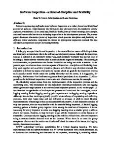
assistance. Other details about the interfaces between subsystems are not provided. The Simultaneous Engineering Workstation (SEW), built at the University of Abertay Dundee, integrates design-byfeature with automated feature-based process planning and NC-code generation [33]. 3. FBICS architecture The FBICS controller hierarchy, shown in Fig. 1, is generally as described in RCS literature. In stand-alone FBICS, levels of controller are included at the RCS Cell, Workstation, and Task levels. In integrated FBICS, additional levels (Elementary move, Primitive, and Servo) are also present. Each controller runs in a separate process or processes (in the operating system sense). Processes may be on the same computer or different computers. Controllers communicate via a messaging system. This hierarchy corresponds to the way many large machine shops actually run. The shop is divided into groups
of machines, each called a cell. A cell is expected to be able to make and inspect a ®nished part from a starting workpiece. A cell includes several workstations. Each workstation has a principal machine and, possibly, auxiliary machines. Each machine can perform several types of task, each task is composed of several elementary moves, each elementary move is decomposed into primitive motions, and each primitive motion is controlled by a servo system. In addition to the controllers, a Solid Modeling Server (Modeler, for short), a Data Repository, and a Graphic Display are included. The Modeler works for the planners, in the Cell, Workstation, and Task controllers. The Graphic Display is connected directly only to the Modeler. Commands for displaying solid objects are available to the three planners, but they are addressed to the Modeler. The FBICS architecture is designed to allow for human participation at every signi®cant step of the process. Elements of this include using appropriate data types at each interface between control levels, having an open ®le format for all data types passing across interfaces, having
658
T.R. Kramer et al. / Computer-Aided Design 33 (2001) 653±669
Fig. 1. FBICS stand-alone architecture.
variable planning depth, and allowing either off-line or online planning. The user-friendly editors and interfaces required for effective human participation in FBICS activities, however, have not been built. The notion of a `set up' is central to FBICS. A setup is a ®xturing of a workpiece on the table of a machining center or coordinate measuring machining. The workpiece does not move with respect to its ®xturing during a single setup. It does move from one setup to the next. Some parts can be handled in a single setup, but more commonly, two or more setups are required.
The ALPS process plan language is used for plans at the Cell and Workstation levels. The fundamental object of ALPS is the plan. A plan is a recipe for performing a speci®c task. A plan in ALPS is a one-level breakdown of a task into subtasks, expressing the requirements of each subtask and its interrelation with other subtasks in the plan. A plan contains a set of nodes (or steps) which provide sequencing information and detail how to perform the task in terms of individual subtasks. Every plan has an associated target system which may execute the plan. ALPS provides for parallel operations, alternatives, synchronization of events,
T.R. Kramer et al. / Computer-Aided Design 33 (2001) 653±669
parameters, and resource allocation. To make ALPS usable in FBICS, two suites of subtypes of the ALPS primitive_task_node have been added to ALPS. One suite, for the Workstation level, is discussed in Section 5. The other suite, for the Cell level, includes only one subtype: run_setup. The stand-alone FBICS architecture is shown in Fig. 1. In stand-alone FBICS, emphasis has been placed on the planning component of each controller. A clean, small, function call interface has been de®ned for each planner, to be used by the rest of the controller. In the stand-alone version, the rest of each controller includes only enough functionality to make the system run and to help with debugging during development. Fig. 1 shows only one subordinate for each superior controller, since that is how stand-alone FBICS is built. In general, in RCS, each superior controller may have several subordinates. The FBICS Task-level controller might be readily split into two task-level controllers, one for a machining center and one for a coordinate measuring machine, for example. The `command message' arrows on Fig. 1 show the direction of ¯ow of commands. In every case (although no return arrows are drawn), a status message ¯ows back to the issuer of the command. Almost all the status messages are simple, meaning `I did it', or `I could not do it.' Status messages from the Solid Modeling Server may be more meaty. Many of them include a Boolean yes/no answer to a question, some include a single numerical value, and others include several related values.
3.3. Task Controller
3.1. Cell Controller
3.4. Solid modeling server
The (top-level) Cell Controller is focused on making a part from a part blank or on inspecting an entire previously made part. The Cell Controller can (1) make a Cell-level process plan for the part, (2) execute a Cell-level process plan, (3) give planning commands to the Workstation Controller, and (4) give execution commands to the Workstation Controller. 3.2. Workstation Controller The (second-level) Workstation Controller handles a single setup of the part (i.e. processing the part without moving it). The Workstation Controller focuses on transforming a workpiece from an incoming shape to an outgoing shape, possibly with intermittent inspection, or on inspecting those features that may be inspected in a single setup. The Workstation Controller can (1) make a Workstationlevel process plan for one setup, (2) execute a Workstation-level process plan, (3) give planning commands to the Task Controller, and (4) give execution commands to the Task Controller.
659
The (third-level) Task Controller focuses on making or inspecting single features. The Task Controller can make a Task-level process plan for machining one feature or inspecting one feature. At the Task level, a machining process plan is an NC-code ®le (in the RS274 language), and an inspection plan is an inspection code ®le (in the DMIS language). The Task Controller can execute Tasklevel plans. In stand-alone FBICS, the Task Planner is split between two processes. The Fbics_Task2 process contains the parts of the planner that run during plan execution. During execution, the Fbics_Task process sends messages to the Fbics_Task2 process, telling it to run a ®le of RS274 code or DMIS code. Splitting the planner between two processes was originally done for convenience. The split has been kept in stand-alone FBICS so that loose integrations are easy to build. In the loose integration that has been used most, messages that would be sent to the Fbics_Task2 process in the stand-alone are redirected to another Tasklevel controller. The FBICS_Task2 process includes version three of the NIST DMIS interpreter and version three of the 3-axis NIST RS274/NGC interpreter. The two messages Fbics_Task2 understands are `run a DMIS ®le' and `run an NC ®le'. In response to these messages, the appropriate interpreter reads the ®le and executes the instructions in the ®le. In the stand-alone version, this results in some degree of emulation of machining or inspection.
The Solid Modeling Server (often shortened to `Modeler' in this document) provides solid modeling services to its clients, which are the controllers. The Modeler maintains a separate view of the shape of objects for each client. The types of service the Modeler provides include, for example, maintaining a model of the current shape of the part, faceting a model and telling the Graphic Display to show it, and determining if a candidate touch point for probing is present on the current part. The Parasolid solid modeler serves as the underlying modeling engine. 3.5. Graphic Display The Graphic Display shows 2D views of 3D objects on a color monitor, using the `movie camera' paradigm [34]. Display of objects is handled by the Modeler and Graphic Display jointly. For each type of object to display, the Modeler facets the object, writes a modeling ®le and sends a message to the Graphic Display, telling the Graphic Display to read the ®le and display it as directed by the user. The display serves to let the user see how planning or execution is progressing. The display is manipulable by the user in the usual ways: move around the object; zoom in or out, etc.
660
T.R. Kramer et al. / Computer-Aided Design 33 (2001) 653±669
The types of object which can be shown are: intended outgoing part shape; incoming part shape; current part shape; feature shape; feature access volume; and ®xture shape. Each object type may be displayed as a solid object, as a wire frame, or not at allÐunder immediate control of the user. The HOOPS graphics system is the underlying graphics engine. 3.6. Data Repository FBICS uses a ®le system as the Data Repository. Data in the repository includes, for example, part designs, process plans, and user option ®les. During FBICS operation, data ®les are written by one process and read by others. Data ®les are used as a supplement to messaging for sending commands from one controller to another. Using a ®le system as the Data Repository has been fully adequate. As FBICS matures it may become desirable to use a database system for the Data Repository, but the need has not yet arisen. 3.7. Interfaces between FBICS modules An FBICS module is a set of related computer code for performing functions of the system. FBICS uses three types of interfaces between modules: application programming interfaces (APIs); messaging interfaces; and ®le interfaces. An API is a set of functions calls available for use between modules. A messaging interface is a set of messages that may be sent between processes by interprocess communication methods. A ®le interface is a set of ®le types which may be written by one process and read by another. For interprocess communication, FBICS uses a messaging interface in every case [35], with most of them being supplemented by a ®le interface. The Cell, Workstation, and Task planners in FBICS each have an API for calls to the planner. The DMIS and RS274/ NGC interpreters included in the Fbics_Task2 process have APIs. The Modeler has an API interface, but, since the Modeler is in a separate process, its API is wrapped in messaging interface. All interfaces between modules are documented in detail in Ref. [1], except the interpreter interfaces, which are explained in Refs. [11,12]. 3.8. User interfaces As shown in Fig. 1, stand-alone FBICS has user interfaces to the three controllers and to the Graphic Display. The user interface to the Graphic Display has the capabilities mentioned above and is totally mouse-driven. The standalone version's user interfaces to the controllers are all simple text-based interfaces that allow the user to exercise the two principal functions of the controller: plan or execute.
3.9. Integrated FBICS Loosely-integrated versions of FBICS have been built with all upper-level components as just described, except for Fbics_Task2. For a loosely-integrated version, the Fbics_Task2 process is replaced by a fully functional RCS controller that includes an RS274 interpreter and/or a DMIS interpreter. For an integration with inspection, the message interface between Fbics_Task and Fbics_Task2 is used unaltered. For an integration with machining, the interface is modi®ed. The fully functional RCS controllers control actual hardware for cutting or inspection [36]. A proposed architecture for tightly-integrated versions of FBICS is described in Ref. [1].
4. Two-stage planning FBICS employs two-stage planning at the Cell, Workstation and Task levels. The use of two-stage planning is driven by the desirability of using ¯exible plans, combined with the requirement of doing hierarchical planning. A ¯exible plan is a plan with variables, alternatives, and (possibly) omissions. Omissions might include omitting tool-changing and coolant commands from stage-one plans; FBICS makes these omissions. Using ¯exible plans solves the common problem that in the discrete parts and other domains where the formulation of plans is costly in time or money, it is desirable that process plans be reusable. If conditions under which plans are executed may change in a way that affects the utility of plans, however, completely ®xed process plans may not be reusable. At least four types of data may change: (1) sensory dataÐ e.g. temperature; (2) resource dataÐe.g. the tools in a machine carousel; (3) job dataÐe.g. the number of widgets to make now; and (4) planning system behavior dataÐe.g. which rule to use to set feed rates. If any of these types of data affects planning, a ®xed plan will become obsolete when the data changes. In FBICS, the stage-one plans prepared in the Cell and Workstation planners are ¯exible plans written in ALPS. A ¯exible plan is expected to be usable for an extended time under a variety of conditions whose variability is embodied in the variables and omissions of the plan. In addition to providing for changeable conditions, a stage-one plan may leave alternatives open because the planning system recognized alternatives but elected not to choose among them. When all alternatives seem equally desirable to a planner, rather than making an arbitrary decision, it seems a better strategy to defer making a decision. Then an executor with better information or a stronger opinion will have the opportunity to exercise its judgement. A stage-one plan may be executed directly. When the plan is executed, it is traversed one step at a time. For each step of the plan, one or more executable operations are executed (by physical action or by sending commands
T.R. Kramer et al. / Computer-Aided Design 33 (2001) 653±669
to a subordinate). By waiting for each command to be executed before selecting the next step to run, the executor allows for using up-to-date values of plan variables. In FBICS, each executable operation is executed by ®rst telling the subordinate to make a plan to carry out the operation and then telling the subordinate to execute the plan it just made. If either the subordinate's planning or its execution is unsuccessful at any point, execution of the superior's plan fails and is stopped. A disadvantage of executing a ¯exible plan directly is that, for each command sent to a subordinate, it may be necessary for the subordinate to make a plan from scratch for carrying out a command received from its superior. If the subordinate planner cannot make such a plan, execution of the superior plan fails. A second disadvantage of executing a ¯exible plan directly is that, if it is executed more than once under the same conditions, after the ®rst execution, the subordinate will be needlessly making the same plans over again, entailing needless cost. If conditions will not change for a period of time during which the superior's plan is to be executed one or more times, it is, therefore, useful to prepare a stagetwo plan for the superior and a set of stage-one plans in the subordinate. To do this, the superior's stage-one plan is traversed, producing a set of executable operations by selecting a speci®c sequence of tasks from among alternatives in the stage-one plan, selecting speci®c resources where the stage-one plan has generic resources, and ®lling in blanks where the stage-one plan has omitted items. The subordinate makes a plan for carrying out each of the superior's executable operations. The superior makes an ordered list of pairs, one for each of the executable operations. Each pair consists of the subordinate plan name and the name of the type of executable operation. This list is the stage-two plan for the superior. FBICS Cell and Workstation-level stage-two plans are modeled very simply and do not use ALPS. Modeling stage-two plans in ALPS would be easily done but cumbersome. Another reason for having stage-two plans is to support optimizing plans across a hierarchy. To perform optimization over a hierarchy via standard search methods, a stage-one plan allowing for all cases to be tested is prepared for the top controller. Partial search plans (plan traversals) are constructed through this top-level plan. For each node (plan step) on a partial search path at the top level, the next level down is told to ®nd an optimum execution. The total cost of any one search path at the top level is the direct cost of the path to the top level plus the cost of each node on the path to the subordinate(s) that handles it. The subordinate controllers follow exactly the same procedure in determining their own optimums. To support this type of search, it is necessary to have a format for recording the optimum path. The stage-two plan provides that format.
661
5. FBICS Workstation tasks A suite of tasks has been de®ned to be used in ALPS stage-one process plans at the FBICS Workstation level. These tasks are the leaf nodes of the supertype-subtype tree shown in Fig. 2. The tasks are divided into two main subtypes: two for inspection and 16 for machining. In the ®gure, the root of the tree is the ALPS primitive_task_node. This is actually a leaf node in the generic ALPS supertypesubtype tree, which is not shown. In Fig. 2, tasks are shown in boldface type. Supertypes are connected to subtypes by lines, with the supertype higher on the page. Attribute names are shown in italic type. Data types of attributes are not shown. Only leaf nodes may be instantiated. To ®nd all attributes of a task, trace down the tree from `primitive_task_node' to the task, and include the attributes of every node along the path, in order. Each task includes a pointer to an AP 224 feature on which the task is to be performed. The form of the pointer is the index number of the feature from the list of features included in the features ®le used in the same setup as the process plan. The attribute containing the pointer is named removal_volume_index. The two subtypes of inspection_task are inspect_feature_surface and inspect_feature_geometry. Only inspect_feature_geometry has been implemented. Of the machining tasks, FBICS currently handles counterboring, ®nish_mill (for rectangular pockets), ®nish_mill_adaptive, and twist_drill. For stage-two Workstation plans, 24 types of executable operation are de®ned. Seventeen of these correspond oneto-one with 17 stage-one tasksÐall but ®nish_mill_adaptive, whose execution requires three executable operations (®nish_mill, inspect, ®nish_mill). The other seven executable operations include coolant control for machining, and three matching pairs (one for inspection and one for machining) for starting a program, changing a tool, and stopping a program.
6. FBICS data ®les All the data languages employed by FBICS are textbased, using ASCII characters; no binary formats are used. Two types of languages are used: those described using STEP with semantics in EXPRESS; and grammar and syntax from STEP Part 21, and those (such as DMIS and RS274) described in a single speci®cation covering semantics, syntax and grammar. Table 2 shows all the ®le types used in FBICS. All ®les except the four marked No EXPRESS Schema are STEP Part 21 ®les corresponding to the schemas listed in Table 2. STEP AP 203 and AP 224 are ISO standards. The tool catalog is being standardized in ISO. The four types not modeled in EXPRESS are DMIS input format,
662
T.R. Kramer et al. / Computer-Aided Design 33 (2001) 653±669
Fig. 2. Workstation-level tasks.
DMIS output format, RS274, and the graphics ®le format. 7. FBICS operation This section describes (1) what happens during FBICS initialization, (2) how planning three levels deep for machining with inspection is done, (3) what the special problems of inspection planning are, (4) what happens during execution of the Cell-level stage-one plan made in item 2, and (5) how adaptive machining has been implemented. 7.1. FBICS initialization FBICS is brought to a warm state when the user gives the shell command `fbics' in a terminal window. This starts the various independent processes and establishes communications among them. FBICS is initialized when the user gives an initialization command to the Cell Controller. This causes initialization command messages to be sent down hierarchically, with
each controller in the hierarchy sending an initialize command to its subordinate, and each subordinate sending an OK message to its superior when it has completed its initialization. During initialization, each planner cleans up its world model, sets default values for various world model parameters, and reads various ®les. The Cell Planner reads the shop_options ®le and resets any inspection and machining parameters in its world model that have values in that ®le. The Workstation Planner does the same with the shop_options ®le, but in addition, reads the tool catalog, tool inventory, and tool_usage_rules ®les named in the shop_options ®le. The Task Planner reads the shop_options ®le, the tool inventory and tool catalog ®les, and a task_options ®le. 7.2. Planning three levels deep for machining with inspection The most complex form of FBICS planning occurs when the Cell Controller is told to plan three levels deep including both machining and inspection, so that type of planning is described here. It is assumed that this type of processing will
T.R. Kramer et al. / Computer-Aided Design 33 (2001) 653±669
663
Table 2 FBICS data in ®les Model name
Item modeled
File writers
File readers
EXPRESS schemas
AP203
Fixture
Workstation & Task planners
ap203
AP 224
All 3 planners Workstation & Task planners All 3 planners Workstation Planner Cell Planner Cell Planner Task Planner (Fbics_Task2) Task Planner (Fbics_Task2) Graphic Display
arm224
RS274/NGC Setup Shop options Task options Tool catalog Tool inventory Workstation stage-one plan
Initial workpiece In-process workpiece Final part Features Cell stage-1 plan Cell stage-2 plan Control code for inspection Results of inspection Access volumes, features, ®xture, ®nal part, workpieces Control code for machining Setup Shop options Task options Tool catalog Tool inventory Workstation stage-one plan
User, CAx (i.e. CAD/CAM/ CAE) system User, Cell Planner Cell Planner User, CAx system Cell Planner Cell Planner Cell Planner Task Planner (Fbics_Task) Task Planner (Fbics_Task2) Modeler Task Planner (Fbics_Task) Cell Planner User User User User Workstation Planner
Task Planner (Fbics_Task2) All 3 planners All 3 planners Task Planner Workstation & Task Planners Workstation & Task Planners Workstation Planner
Workstation stage-two plan Workstation executable operations
Workstation stage-two plan Workstation executable operation
Workstation Planner Workstation Planner
Workstation Planner Task Planner
No EXPRESS schema setup shop_options task_options tool_catalog fbics_combo, expressions fbics_combo, fbics_alps, arm224 fbics_combo fbics_combo
Cell Stage-1 Plan Cell Stage-2 Plan DMIS input format DMIS output format Graphics ®le
be performed by a machining center equipped with cutting tools and a touch-trigger probe. Other types of planning for a machining center are similar but simpler, usually including a subset of the three-level planning activities. 7.2.1. Cell controller planning When the user gives a plan_part command to the Cell Controller, the user provides the ®le name of the design of the part to be made, the ®le name of the design of the incoming workpiece, a ¯ag indicating whether the incoming workpiece design ®le already exists or should be written, the base name for setup ®les, the base name for plan ®les, the name of the ®xture ®le to use, and the number of levels to plan. We are assuming here that the number of levels is three. The general plan of attack is to make a stage-one Cell-level plan ®rst, then make a stage-two plan from the stage-one plan, giving planning commands to the Workstation Controller as the stage-two Cell-level plan is made. To make a stage-one plan, the Cell Controller reads the ®les describing the design of the part to be made and the incoming workpiece. The Cell Controller makes a few initial checks, such as requiring that the shape to be made is contained in the incoming workpiece and winnowing down the features to be made by throwing out those whose intersection with the initial workpiece is empty. The set of features to be made is divided into subsets called direction-sets, all of whose native z-axes point in the same direction (since these are all machinable from the same direction). Some of the features to be made will block access to making other features in the same directionset or other direction-sets. Blocking features must be made
fbics_combo, fbics_alps fbics_combo No EXPRESS schema No EXPRESS schema No EXPRESS schema
before blocked features. With the help of the Modeler, an analysis of the blocking situation is made. Using the results of this analysis, the features to be made are assigned to setup-sets (each of which is either an entire direction-set or a subset of a single direction-set) and the setup-sets are partially ordered. The partial ordering is captured in a Celllevel stage-one ALPS process plan. The plan nodes that are partially ordered are all run_setup nodes, one for each setupset. For each run_setup plan node, a meta®le called a setup ®le is made and its name is recorded in the run_setup node. Several data ®les referenced in the setup ®le are made, as well, including (1) a ®le describing the features to be made in the setup, (2) a ®le describing the shape of the workpiece coming into the setup (if there is only one possible such shape), and (3) a ®le describing the shape of the workpiece leaving the setup (if there is only one possible such shape). The names of these additional ®les are recorded in the setup ®le along with the base name of a Workstation plan for making the features, the name of a ®xture ®le, and the direction of the setup-set. To make a stage-two plan, the Cell traverses the stage-one plan. Each plan step the Cell decides to do next is a run_setup step, so one of two types of run_setup operation is put into the stage-two plan. Since three levels are being planned, a run_setup2 operation (indicating a stage-two Workstation plan should be run) is used and a stage-two Workstation plan is named in the operation. Also during the traversal, the Cell determines the shape of the incoming and outgoing workpiece for each setup. If either shape was unknown when the setup ®le for the setup was written, the
664
T.R. Kramer et al. / Computer-Aided Design 33 (2001) 653±669
setup ®le is rewritten and a ®le (or two) describing the previously unknown shape(s) is written. The Cell then commands the Workstation to make a plan two hierarchical levels deep for the (now fully speci®ed) setup. 7.2.2. Workstation controller planning Each time the Cell Controller commands the Workstation Controller to plan a setup two levels deep, the Workstation Controller ®rst makes a stage-one plan for the setup, then makes a stage-two plan from the stage-one plan (generating command ®les to be used later by the Task Controller as it builds its stage-two plan). Finally, the Workstation Controller traverses its stage-two plan. To make a stage-one plan, the Workstation Controller ®rst reads the setup ®le. This tells it what the name of the plan it writes should be, as well as the names of ®les to read. The Workstation Controller reads the ®les and calls on the Modeler to set up solid models of all parts and features in the correct orientation. Then the Workstation Controller analyzes the feature blocking situation and constructs a partial ordering for making the features. It also decides which features are to be inspected. For each feature to be machined, the Workstation Controller selects a machining operation appropriate to make the feature and a type of cutting tool with which to perform the operation. Values are selected for tool use parameters (feed, speed, etc.). For each feature to be inspected, the Workstation Controller selects an inspection operation and a touch-trigger probe with which to perform the operation. To make a stage-two plan, the Workstation Controller traverses the stage-one plan. For each step of the stageone plan the Workstation Controller decides to execute, the Workstation Controller de®nes one or more Task-level operations required to accomplish that step. For each operation, the Workstation Controller writes a ®le describing the operation. Finally, the Workstation Controller traverses the stagetwo plan and, for each operation, sends a planning command to the Task Controller. 7.2.3. Task controller planning When the Task Controller receives an open_setup command, it reads the setup ®le whose name is received with the command, reads the ®les describing the incoming part and ®xture, and calls the Modeler to model the incoming part and ®xture. A generate_nc command includes (1) the name of a ®le describing the machining operation and feature to make and (2) the name of an NC-code ®le to write. When the Task Controller receives a generate_nc command, it reads the input ®le, calls the Modeler to model the feature and the workpiece as it will be when that feature is subtracted from it, and calls an NC-code generator to write the output ®le. A generate_dmis command includes (1) the name of a ®le describing the inspection operation and feature to inspect and (2) the name of a DMIS code ®le to write. When the
Task Controller receives a generate_dmis command, it calls a DMIS code generator to write the output ®le. DMIS generation details are given in Section 7.3.4. The Task Controller does not make stage-two plans. A Task-level stage-two plan would be a list of canonical machining and/or inspection commands as generated by the DMIS and RS274 interpreters. Since sensory data from the next lower control level often affect the generation of canonical commands, pre-generated lists of canonical commands are usually not valid. 7.3. Inspection planning The behavior of the system when planning for pure inspection is much the same as in machining planning. One factor makes inspection planning easier: the workpiece does not continually change shape during processing. A second factor makes inspection planning harder: until it is decided which features are to be inspected, it is not known whether any proposed setup will be required. Thus, the Cell Controller must use the same decision rules as the Workstation Controller while the Cell Controller plans inspection setups. Using the same decision rules is implemented by putting them in the shop_options ®le, which is used by both controllers. In machining planning, deciding what to do is simpleÐ every bit of material in all the features not already on the workpiece has to be removed. In inspection planning, deciding what to do is not so simple. Which AP 224 features should be inspected? How thoroughly should they be inspected? When should they be inspected? The approach to these questions taken in FBICS is that there is no `right' answer, so let the user decide. This is implemented by user preference ®les and (if user preferences specify it) by asking the user on a case-by-case basis. 7.3.1. Which features to inspect Options regarding which features to inspect are used in the Workstation Planner. Five choices are provided in the shop_options ®le: (1) inspect all features; (2) inspect no features; (3) inspect any feature with any parameter having any tolerance; (4) inspect any feature which has any parameter with a tight tolerance; and (5) let the user decide for each feature. The de®nition of what is a `tight' tolerance for milling is another user option. 7.3.2. How thoroughly to inspect a feature It is impossible to inspect every point on a surface, so a decision must be made on which points to inspect. FBICS uses the qualitative idea of high, medium, and low inspection intensity. The user may specify in the task_options ®le how many points to inspect at each of these three levels for each DMIS feature type. 7.3.3. When to inspect FBICS currently inspects each feature immediately after
T.R. Kramer et al. / Computer-Aided Design 33 (2001) 653±669
cutting. This wastes time, since doing it requires that the tool be changed and the coolant turned on or off before and after every cutting operation. For complex parts, waiting to inspect until cutting is complete might also be wasteful, since if any cutting operation spoils the part, all the following cutting operations are wasted effort. An option for how many features to cut before inspecting any features to be inspected has been de®ned and may be included in shop_options ®les, but the information is not used in the current implementation. 7.3.4. DMIS code generation from AP 224 features The DMIS language de®nes a number of surface features. These include plane, cylinder, cone, and sphere, among others. These are simpler than features de®ned in AP 224, which has, for example, pocket and hole. To generate DMIS code from AP 224 features, it is necessary to decompose the surface of each AP 224 feature into a set of DMIS features. The surface of the prototypical AP 224 pocket, for example, may be decomposed into nine DMIS features: ®ve planes (four sides and a bottom) and four cylinders (the corners of the pocketÐeach is a quarter cylinder). For each DMIS feature present in principle, DMIS code is written (1) to de®ne the feature, (2) to measure the feature, and (3) to report the results of the measurement. If the feature is a cylinder with a diameter tolerance (inherited from a tolerance on the corner radius of an AP 224 pocket), DMIS code is also written to de®ne the tolerance, calculate the error in the diameter, and report whether the cylinder diameter is intolerance or not. 7.4. Executing a stage-one cell-level plan This section describes what happens when the user tells FBICS to execute the stage-one Cell-level plan for machining described in Section 7.2. Stage-two plan execution, which is much simpler (essentially: do the operations on the list in order) is not described in this paper, but is in Refs. [4,11]. During execution of a stage-one Cell-level plan, the Cell Controller traverses the plan one step at a time. For each plan step (they are all run_setup steps), the Cell Controller ®rst sends a plan_setup command to the Workstation Controller, and then a run_setup command (indicating a stage-one plan should be used) immediately after. The way in which the Cell Controller traverses its stage-one plan and disambiguates data is identical to the way it is done in preparing a stage-two plan from a stage-one plan (described in Section 7.2.1). A slightly different naming convention is used for the disambiguated data, which is intended to be short-lived in the case of executing a stageone plan. For each plan_setup command it receives, the Workstation Controller makes a stage-one plan exactly as described in Section 7.2.2. For each run_setup (using a stage-one plan) command it receives, the Workstation Controller reads the
665
stage-one plan and traverses the stage-one plan (also exactly as described in Section 7.2.2), writing operations ®les as described in that section. During execution, however, as soon as each operation is selected, the Workstation Controller ®rst sends a generate_nc or generate_dmis command to the Task Controller then sends an execute_nc or execute_dmis command immediately afterwards. Generating NC code and DMIS code in the Task Controller is the same during executing as during planning. Executing the code is done only during execution. As shown in Fig. 1, the Task Controller includes two separate processes. Code generation is performed entirely by the Fbics_Task process. Code execution is performed entirely by the Fbics_Task2 process. For each generate_nc command it receives specifying that an AP 224 feature should be cut, the Task Controller reads the ®le describing the operation and generates the tool path to use to cut the feature. Tool use parameters are given in operation ®les for cutting. Thus, the code that is generated may include commands to reset the values of spindle speed or feed rate. For each generate_dmis command the Task Controller receives specifying that an AP 224 feature should be inspected, the Task Controller generates code as described in Section 7.3.4. For each execute_dmis or execute_nc command the Task Controller receives, the Task Controller (by call to either the DMIS interpreter or the RS274 interpreter) interprets the ®le named in the command, adjusts its internal model appropriately, and makes calls to canonical machining or inspection functions. In stand-alone FBICS, these canonical calls simply print themselves and update a dummy external world model required by the interpreter. In integrated FBICS, the canonical calls are used for machine control and actual cutting or inspection. 7.5. Feedback from inspection to planning FBICS includes using feedback from inspection to planning, as follows. If there is a tight tolerance on any of the length, width, or corner radius of a pocket to be ®nishmilled, the Workstation Planner puts a ®nish_mill_adaptive step for milling the pocket in the stage-one plan. Both a cutting tool and a probe tool are used in the step. Tool-use parameters for both tools are also included. When operations are created for carrying out that step during execution of the plan, three primary operations are de®ned (in addition to tool changing and coolant control, if needed). The ®rst primary operation is to ®nish mill a test pocket in the same place as, but slightly smaller than the speci®ed pocket. The second is to inspect the test pocket, and the third is to ®nish mill the ®nal pocket. When the Task Controller executes the DMIS ®le for inspecting the test pocket, the DMIS interpreter (because the inspection program says to do so) writes a ®le containing the results of the inspection. Before generating code for the ®nal cut on the pocket, the Workstation reads this ®le. A correction factor for the ®nal cut is calculated as the average error in the radii of the four corners of
666
T.R. Kramer et al. / Computer-Aided Design 33 (2001) 653±669
the test pocket. If the test pocket corner radii were too big on average, NC code is written so the ®nal cut is made inside the nominal tool path for the ®nal pocket by the correction factor. If the test pocket radii were too small, NC code is written so that the ®nal cut is outside the nominal path by the correction factor.
2. 3.
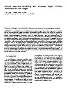
8. Results and a simple example FBICS has been tested successfully with simulated machining and inspection using moderately complex parts, including the much-used ANC101 and TEAM test parts. Integrated tests with machining or inspection have not been as complex. Planning to depth two for machining the 51-feature the TEAM part with in-process inspection of six holes (starting with a featureless block) and executing the plans in simulation results in one Cell plan, Workstation plans for eight setups, 157 NC-code ®les, nine DMIS ®les, and associated data. A total of 373 ®les is written. On a Sun SPARCstation 20, planning the TEAM part took 16 min and execution took 12 min. Over 90% of the time is used in the Modeler and Graphics Display. Results for the ANC101 part are similar. Describing the processing of the TEAM or ANC101 part would take far too much space. This section, therefore, provides a much simpler example of FBICS in action. The example part, `simple_part', is a block with a pocket on top and a hole on one side. A picture of simple_part is shown in Fig. 3. This example involves stage-one plans only. Planning one level deep for simple_part (Cell only) took 15 s on a Sun SPARCstation 20. Executing the Cell plan (which triggers Workstation level planning for two setups, as well as NC-code generation and simulated execution) took 50 s. For simple_part, 41 ®les are written, as summarized in Fig. 3B. An abbreviated description of what happens during planning and execution for simple_part follows. All mention of what the Modeler and Graphics Display do is omitted. Planning for the simple part is started by typing the following command at the user interface for the Cell controller: plan_part(simple_part.stp, OFF, block.stp, plans, feats, ®1, setups, 1). The 1 at the end of this command means that FBICS should plan one level deep (i.e. at the Cell level only). The name of the AP 224 STEP Part 21 ®le giving the design of this part to make is simple_part.stp. The data section of this ®le is shown in Fig. 3A. OFF means that the ®le giving the design of the shape to start with (block.stp) does not yet exist and should be created. plans is the root name for process plan ®les to write (including ALPS, DMIS and RS724 ®les). feats is the root name for feature ®les to write. ®1 is the name of the ®xture to use, which must already exist. setups is the root name for setups to write. To carry out this command, the Cell planner: 1. Reads simple_part.stp and builds a `feature_plus'Ða
4.
5.
structure with additional data about the featureÐfor each feature of simple_part. Creates the starting shape for machining by making a copy of the base shape of simple_part and writes the ®le block.stp. Divides the features into sets which may be made in one setup and puts the sets into batches which may be in any order. In the case of simple_part there are two sets (each containing one feature) and one batch (containing both sets). Makes a Cell-level stage-one plan and prints it to the ®le plans_1cell.stp. The data section of this ®le and the graph of the plan are shown in Fig. 3C and D. The plan indicates that the two setups may be made in any order. Makes a setup ®le for each of the two setup, setups_1.stp and setups_2.stp. The structure (not the text) of setups_2.stp is shown in Fig. 3E. The setups_1.stp ®le is similar. Because the two setups may be made in any order, it is not known what the incoming or outgoing part will be for either setup (hence the `not_set' entries in Fig. 3E), although it is known what features will be made during each setup. The setup ®le positions the part_in, part_out, and features with respect to the working coordinate system of the machine so that the axis of the hole to be drilled is vertical and the features (i.e. the hole), part_in and part_out are in the correct relative location. The ®xture is in the same location for both setups. The base name, `plans_2.stp', for the Workstation-level and Task-level plans is known, even though they have not yet been written.
To execute the plan plans_1cell.stp, the user types at the user interface for the Cell Controller: run_part1(plans). In response: 1. The Cell reads the ®le plans_1cell.stp and starts traversing the plan graph (shown in Fig. 3D). When it comes to the split node (item 2 in Fig. 3D), it decides to process node 3 (run the ®rst setup) ®rst. 2. The Cell reads the ®le setups_1.stp. Since it knows from its plan that the part_in for the entire process is `block.stp' and it knows this is the ®rst setup, it replaces the `not_set' part_in for the ®rst setup with `block.stp'. It also changes the part_out in the ®rst setup from `not_set' to `simple_part_temp_1.stp'. It then writes setups_1_temp.stp, a revised version of setups_1.stp. 3. The Cell sends a command message to the Workstation telling it to make a plan for executing the ®rst setup as speci®ed by setups_1_temp.stp. 4. The Workstation, on receiving this message, reads setups_1_temp.stp and all the ®les it names. Then it makes a stage-one plan for doing the work speci®ed by the setup and sends a done status message to the Cell. The plan it makes is very simple, since there is only one feature to makeÐjust start, mill a pocket, and end. It writes this plan in the ®le plans_1_1work.stp.
T.R. Kramer et al. / Computer-Aided Design 33 (2001) 653±669
667
Fig. 3. Simple example.
The node to mill a pocket includes the name of the type of tool to use, the feed rate, the spindle speed, the horizontal stepover to use, and the vertical pass depth. The plan includes the name of the setup ®le. 5. The Cell, on learning that the Workstation has completed planning for the ®rst setup, sends a command message to the Workstation telling it to execute that plan. 6. The Workstation, on receiving this message, reads the ®le plans_1_1work.stp, the ®le setups_1_temp.stp, and the ®les named in that setup ®le. The Workstation sends an open setup command message to the Task, which reads the setup ®le and gets ready to run. This implicitly
includes ®xturing the workpiece as speci®ed by the setup ®le. 7. The Workstation starts traversing the (start-mill-end) plan graph. Traversing the start node results only in checking. When the mill node is reached, the Workstation plans four executable operations to carry out that node: start_nc; change tool; adjust coolant (on); and ®nish_mill. It then executes these operations in order. Executing the last of the operations results in the pocket being milled. For any operation requiring a tool, a speci®c tool is selected from the tool inventory. The method of executing an operation is described immediately following.
668
T.R. Kramer et al. / Computer-Aided Design 33 (2001) 653±669
8. To execute an operation, the Workstation ®rst writes a command ®le, and then sends a command message to the Task, telling it to generate NC code and giving it the name of the command ®le. The data section of a sample command ®le (for the hole drilling operation that occurs later) is shown in Fig. 3F. Each command ®le describes the operation and the plan step that gave rise to the operation. If the operation is performed on a feature (as the ®nish milling operation is performed on a pocket, for example) the command ®le also describes the feature. The Task, on receiving the message, generates an NCcode ®le and returns a done status message. The Workstation then sends an execute_nc message to the Task, telling it to execute the NC code, which the Task does. 9. The Workstation next handles the end node of its plan, for which it generates two operations, adjust coolant (off) and end_nc. These are executed by Task as described immediately above. That completes execution of the Workstation plan for the ®rst setup. The Workstation then sends a done status message to the Cell. 10. The Cell continues to traverse its plan, ®rst going back to the split node (to see what might be done next) and then deciding to do the second run_setup (item 4 in Fig. 3D). The process outlined in paragraphs 2±9 above is repeated for the second setup, resulting in the hole being drilled. Then the Cell ®nishes traversing its plan, cleans up, and is ready to do something else.
[4] [5] [6] [7] [8]
[9] [10] [11] [12] [13]
[14]
[15]
9. Conclusion The FBICS architecture provides for planning and control of machining and inspection of discrete parts in a hierarchical control system. The FBICS implementations demonstrate that the architecture, including its speci®c modularization of manufacturing activities, is usable for industrial application. The implementations also demonstrate the feasibility of feature-based manufacturing and the usability of the ALPS process planning language, STEP AP 224, and STEP data handling techniques and tools, generally. FBICS demonstrates the feasibility and desirability of two-stage planning. FBICS is unusualÐ possibly uniqueÐin (i) its ability to generate plans for several levels of a hierarchical control system, (ii) its implementation of two-stage planning, and (iii) its use of STEP AP 224 for part modeling.
[16] [17] [18] [19] [20] [21] [22] [23] [24]
References [1] Kramer TR, Huang H-M, Messina E, Proctor FM, Scott H. Featurebased inspection and control system. NISTIR, 2000 (in draft). [2] Proctor FM, Kramer TR. A feature-based machining system using STEP. Proceedings of SPIE Conference on Sensors and Controls for Intelligent Machining, Agile Manufacturing, and Mechatronics, November, Boston, MA. SPIE 1998;3518:156±63. [3] Messina E, Horst J, Kramer T, Huang H, Tsai T, Amatucci E. A
[25]
[26] [27]
knowledge-based inspection workstation. Proceedings of the IEEE International Conference on Information, Intelligence, and Systems, Bethesda, MD, 1999. Kramer TR, Huang H-M, Messina E, Proctor FM, Scott H. An automatic hierarchical process planning system, 2000 (in draft). Albus JS. A theory of intelligent systems. Control and Dynamic Systems 1991;45:197±248. Albus JS, McCain HG, Lumia R. NASA/NBS standard reference model for telerobot control system architecture (NASREM): NIST Technical Note 1235. ed. NIST 1989:1989. Albus JS. A reference model architecture for intelligent systems design, NISTIR 5502. NIST, 1994. Electronic Industries Association. EIA Standard EIA-274-D interchangeable variable block data format for positioning, contouring, and contouring/positioning numerically controlled machines. Washington, DC: Electronic Industries Association, 1979. National Center for Manufacturing Sciences. The next generation controller part programming functional speci®cation (RS-274/ NGC), draft. NCMS, 1994. Consortium for Advanced ManufacturingÐInternational. Dimensional measuring interface standard; revision 3.0, ANSI/CAM-I 101-1995. Arlington, TX: CAM-I, 1995. Kramer TR, Proctor FM. The NIST RS274/NGC interpreter version 2, NISTIR 5739. NIST, 1995. Kramer TR, Proctor FM, Rippey WG, Scott H. The NIST DMIS interpreter version 2, NISTIR 6252. NIST, 1998. Proctor FM et al. Simulation and implementation of an open architecture controller. Proceedings of the SPIE International Symposium on Intelligent Systems and Advanced Manufacturing, Philadelphia, PA, 1995. Kramer TR, Jun J-S. Software for an automated machining workstation. Proceedings of the International Machine Tool Technical Conference. Chicago, IL: National Machine Tool Builders Association, 1986. p. 1986;12-9:12±44. Kramer TR. The off-line programming system (OLPS): a prototype STEP-based NC-program generator. Proceedings of a Seminar (Product Data Exchange for the 1990s), vol. 2. New Orleans, LA: NCGA, 1991 Kramer TR. A library of material removal shape element volumes (MRSEVs), NISTIR 4809. NIST, 1992. Kramer TR, Proctor FM. Feature-based control of a machining center, NISTIR 5926. NIST, 1996. Albus J.S., et al. NIST support to the next generation controller program. ®nal technical report, 4888. NIST, 1992. Proctor FM, Kramer TR. Canonical machining commands, NISTIR 5970. NIST, 1997. Catron B, Ray SR. ALPSÐA language for process speci®cation. International Journal of Computer Integrated Manufacturing 1991;4(2):105±13. Wallace S, Senehi MK, Barkmeyer E, Ray S, Wallace EK. Control entity interface speci®cation, NISTIR 5272. NIST, 1993. Jurrens KK, Fowler JE, Algeo ME. Modeling of manufacturing resource information, NISTIR 5707. NIST, 1995. ISO 10303-11: Industrial automation systems and integrationÐ product data representation and exchange±Part 11: the EXPRESS language reference manual. Geneva, Switzerland: ISO 1994:1994. ISO 10303-21: Industrial automation systems and integrationÐ product data representation and exchangeÐPart 21: clear text encoding of the exchange structure. Geneva, Switzerland: ISO 1994:1994. ISO 10303-224: Industrial automation systems and integrationÐ product data representation and exchangeÐPart 224: application protocol: mechanical product de®nition for process planning using machining features. Geneva, Switzerland: ISO 1998:1998. Anderson DC, Chang TC. Geometric reasoning in feature based design and process planning. Computers & Graphics an International Journal 1990;14(2):225±35. Anderson DC, Chang TC. Automated process planning using
T.R. Kramer et al. / Computer-Aided Design 33 (2001) 653±669
[28] [29] [30] [31] [32] [33] [34] [35] [36]
object-oriented feature based design; advanced geometric modelling for engineering applications. North-Holland, 1990. Anderson D. Purdue quick turnaround cell. http://cadlab.www.ecn.purdue.edu/qtcplm 1999. http://cybercut.berkeley.edu U. C. Berkeley Cybercut website. Smith CS, Wright PK. Cybercut: a World Wide Web based design-tofabrication tool. Journal of Manufacturing Systems 1996;15(6):432±42. Wang F-CF, Wright PK, Web-based CAD. tools for a networked manufacturing service. Proc. of the ASME Design Engineering Technical Conference, Atlanta, GA 1998:1998. Judd RP et al. The intelligent machining workstation. Prototyping Technology International 3:52±5. Naish JC, Mill FG, Salmon JC. An industry-based study of cutting process capability representation requirements for an integrated engineering workstation. IIE Transactions 1997;29:573±84. Leler W, Merry J. 3D with HOOPS. Addison-Wesley, Reading, MA, 1996. Shackleford W. Real-time control systems library documents. http:// isd.cme.nist.gov/proj/rcs_lib 1996. Horst JA. Real-time and object-oriented issues for an inspection workstation application. Proceedings of the Fifth International Workshop on Object-Oriented Real-Time Dependable Systems, 1999.
669
Elena Messina is the Group Leader of the Knowledge Systems Group in the Intelligent Systems Division at the National Institute of Standards and Technology. She is also Program Manager for Research and Engineering of Intelligent Systems. Her work responsibilities include knowledge representation and planning for control, establishment of performance metrics for intelligent systems, and development of software architectures, tools, and methodologies for building controllers. Current testbeds include an autonomous scout vehicle and an inspection workstation with feature-based planning, control and part localization. Prior to joining NIST, she was Manager of Geometric Modeling for the I-DEAS Master Series CAD/CAE Software at the Structural Dynamics Research Corporation. Ms. Messina also worked at Cincinnati Milacron on their industrial robots, where she received two patents for her arc welding-related enhancements. She received a BS in Engineering Science from the University of Cincinnati.
Thomas Kramer is a Guest Researcher in the Intelligent Systems Division at the National Institute of Standards and Technology and a Research Associate of the Catholic University of America. He has worked full-time at NIST since 1984. Mr. Kramer has been developing concepts and software for feature-based manufacturing systems since 1986. His primary research interest is automated reasoning. At NIST he has also worked on control architectures, interpreters for machine control languages, and data standards related to manufacturing. He received a BA in Physics from Swarthmore College in 1965 and an MA and PhD in Mathematics from Duke University in 1968 and 1971, respectively.
Harry Scott is the project manager for the Reference Model Architecture project within the Manufacturing Engineering Lab at NIST. This program addresses interoperability issues in intelligent control systems, in part, through the development and testing of a reference model for design and implementation of realtime, intelligent systems. Prior work has included integration of the Inspection Workstation Testbed into the National Advanced Manufacturing Testbed (NAMT) CIM Framework, wireless communication system implementations for DOD and DOT intelligent vehicle programs, a DOT investigation into vehicle-to-roadside communication technologies, and control system development and integration for the Advanced Manufacturing Research Facility at NIST in the 1980s. Mr. Scott holds a BS in Electrical Engineering from the University of Maryland.
Hui-Min Huang is a Mechanical Engineer with the National Institute of Standards and Technology (NIST), US Department of Commerce. His major research areas include the architectures and software engineering tools and methodologies for real-time, intelligent control systems. His prior professional experiences include technical positions with the Advanced Technology and Research Company (Burtonsville, MD), the Singer Company Link Simulation Division (Silver Spring, MD) and the Timex Watches Company (Taiwan). Mr. Huang received an MS degree in Mechanical Engineering from the University of Texas at Arlington in 1982 and an MS degree in Computer Science from the Johns Hopkins University in 1986.
Frederick Proctor is the Group Leader of the Control Systems Group at the National Institute of Standards and Technology. He received a BS in Electrical Engineering from the Univesity of Maryland in 1986, and an MS in Computer Science from the John Hopkins Univesity in 1993. His research interests include control of manufacturing systems, real-time software, and validation testing for open architecture control standardization. Recently, Mr. Proctor has been contributing to an open-source project on computer numerical control and programmable logic controllers, in collaboration with small manufacturers.