A Finite-Differences Derivative-Descent Approach for Estimating Form Error in Precision-Manufactured Parts Abhijit Gosavi Assistant Professor e-mail:
[email protected]
Shantanu Phatakwala Research Assistant Department of Industrial Engineering, University of Buffalo, State University of New York, 317 Bell Hall, Buffalo, NY 14260-2050
Background: Form-error measurement is mandatory for the quality assurance of manufactured parts and plays a critical role in precision engineering. There is now a significant literature on analytical methods of form-error measurement, which either use mathematical properties of the relevant objective function or develop a surrogate for the objective function that is more suitable in optimization. On the other hand, computational or numerical methods, which only require the numeric values of the objective function, are less studied in the literature on form-error metrology. Method of Approach: In this paper, we develop a methodology based on the theory of finite-differences derivative descent, which is of a computational nature, for measuring form error in a wide spectrum of features, including straightness, flatness, circularity, sphericity, and cylindricity. For measuring form-error in cylindricity, we also develop a mathematical model that can be used suitably in any computational technique. A goal of this research is to critically evaluate the performance of two computational methods, namely finite-differences and Nelder-Mead, in form-error metrology. Results: Empirically, we find encouraging evidence with the finite-differences approach. Many of the data sets used in experimentation are from the literature. We show that the finite-differences approach outperforms the Nelder-Mead technique in sphericity and cylindricity. Conclusions: Our encouraging empirical evidence with computational methods (like finite differences) indicates that these methods may require closer research attention in the future as the need for more accurate methods increases. A general conclusion from our work is that when analytical methods are unavailable, computational techniques form an efficient route for solving these problems. 关DOI: 10.1115/1.2124989兴 Keywords: form error, metrology, derivative descent, finite differences, cylindricity
1
Introduction
Quality assurance of parts manufactured in the industry usually requires that they conform to tolerance specifications, which may be internal or customer-specified. According to a modern perspective, quality is inversely proportional to variation 关1兴. To reduce variation, it becomes necessary to measure variation accurately in Contributed by the Manufacturing Engineering Division of ASME for publication in the JOURNAL OF MANUFACTURING SCIENCE AND ENGINEERING. Manuscript received November 10, 2004; final manuscript received April 5, 2005. Review conducted by T. R. Kurfess.
the first place. Measurement of form errors was carried out in the early days of manufacturing with mechanical instruments. In modern times, Coordinate Measuring Machines 共CMMs兲 are used quite heavily, although for certain types of measurements mechanical devices such as gauges and V-blocks 关2兴 are popular to this day. CMMs have made it possible to gather large sets of data—from the surface of the part to be measured—allowing increased accuracy in the measurement performed. This, and the fact that the power of modern-day computers has increased dramatically, have enabled the processing of large amounts of data with complex algorithms. In this paper, we focus on computational methods for surfacemetrology features belonging to the class of form errors. Examples of such features are: Straightness, flatness, circularity, sphericity, and cylindricity. While there has been a large volume of work in analytical methods for form-error measurement, computational methods have received less attention in the literature. Analytical methods exploit mathematical properties of the relevant objective function for optimization or optimize a surrogate objective function. Contrary to this approach, computational methods use numeric values of the objective function for optimization. Computational methods become attractive when it is difficult to obtain optimization-oriented, analytic properties of the objective function without tampering with it. In this paper, we introduce the method of derivative descent in the form of finite differences, which makes it a computational approach, for measurement of form errors. We also derive a model for measuring form error in cylindricity; the model can be used suitably in any computational technique. And finally, we test the performance of the finite-differences approach and a Nelder-Mead approach on numerous data sets—some of which are from the literature— related to all of the form-error features enumerated above. The empirical evidence that we have gathered suggests that for more complex features such as sphericity and cylindricity, the finitedifference approach outperforms the Nelder-Mead approach; of course, both techniques consistently outperform the least-squares technique that is widely used in industrial software. The rest of this paper is organized as follows. Section 2 provides the background material for this subject along with the derivation of the form useful in determining cylindricity errors. Section 3 presents the finite-differences derivative-descent approach. Computational experiments are reported in Sec. 4. Section 5 concludes this paper with a discussion on topics related to future research.
2
Background
In this section, we will first define form-errors for straightness, flatness, circularity, and sphericity. For cylindricity, we will devise the closed form required for cylindricity error. Thereafter, we will also present the formulations used in least-squares techniques. 2.1 Form-Error Features. The ith data point on the surface being inspected will be denoted either by 共xi , y i兲 or 共xi , y i , zi兲 depending on whether two-dimensional or three-dimensional data are required, where for the ith point, xi , y i, and zi denote the x , y, and the z coordinates, respectively. To model the straightness error, we define a straight line using: y = mx + c where m and c are the defining parameters of the equation. The vertical deviation of a point, 共xi , y i兲, on the edge from the reference form is: ei = y i − 共mxi + c兲. This deviation is measured along the y axis. The normal deviation of the same point from the reference edge is given by: ei = 共y i − 共mxi + c兲兲 / 冑1 + m2. Vertical deviations are more easily minimized than normal deviations using the popular least-squares method, which we will discuss later, and hence have been used extensively in commercial software. However, it is the normal deviation that measures the actual deviation according to Refs. 关3–5兴. Unfortunately, normality introduces nonlinearity in the definition of error, making its analysis more complicated. Flatness is an extension of straightness to 3 dimensions. The
Journal of Manufacturing Science and Engineering Copyright © 2006 by ASME
FEBRUARY 2006, Vol. 128 / 355
Downloaded 08 Sep 2008 to 131.151.83.65. Redistribution subject to ASME license or copyright; see http://www.asme.org/terms/Terms_Use.cfm
Fig. 1 A 2-step procedure in form-error measurement
equation of a plane is defined as: z = mx + ly + c. The normal deviation of any measured point, 共xi , y i , zi兲, from the reference plane is given by: ei = 共zi − 共mxi + ly i + c兲兲 / 冑共1 + m2 + l2兲 and the vertical deviation is given by: ei = zi − 共mxi + ly i + c兲, which is measured along the z axis. For defining circularity 共or roundness兲, we need to define a circle whose equation is 共x − a兲2 + 共y − b兲2 = R2 where R is the radius of circle and the coordinates of the center of the circle are: 共a , b兲. The defining parameters of the equation of a circle are thus: a , b, and R. Unlike straightness or flatness, for circularity, only one type of deviation is of interest, which is called the radial deviation. The latter is measured along the radius from the circle center to the point in question. Hence the radial deviation for a point, 共xi , y i兲, is: ei = 冑共xi − a兲2 + 共y i − b兲2 − R in which the squarerooted term is the distance from 共xi , y i兲 to the circle’s center. The equation of a sphere is given as: 共x − a兲2 + 共y − b兲2 + 共z − c兲2 = R2, where R is the radius of the sphere and the sphere’s center is: 共a , b , c兲. The radial deviation for sphericity, which is an extension of the same for circularity to three dimensions, is defined as: ei = 冑共xi − a兲2 + 共y i − b兲2 + 共zi − c兲2 − R. The defining parameters of the equation of a sphere are thus: a , b , c, and R. In the deviation, the square-rooted term is the distance from 共xi , y i , zi兲 to the center of the sphere. For measuring cylindricity, we will employ a cylinder whose radius is R and whose axis is given by: x−u y−v z−w = = . m l k
共1兲
Then the defining parameters of its equation are: l , m , k , u , v , w, and R. The deviation of any point on a real cylinder from a perfect cylinder can then be shown to be: ei = 冑共xi − mti − u兲2 + 共y i − lti − v兲2 + 共zi − kti − w兲2 − R, in which ti =
共2兲
共xi − u兲m + 共y i − v兲l + 共zi − w兲k . m2 + l2 + k2
共3兲
In Eq. 共2兲, the square-rooted term is the normal distance from a point, 共xi , y i , zi兲, on the surface of the cylinder, to the axis of the cylinder. We now provide a proof of the validity of the model presented above. ជ denote a vector whose one Derivation of Eq. (2) and (3): Let end point is 共xi , y i , zi兲 and the other is on the axis of the cylinder, and the vector itself is perpendicular to the axis. Now, from the definition of the axis, i.e., Eq. 共1兲, 共m , l , k兲 is a vector on the axis. ជ and 共m , l , k兲 has to be zero. Now, let Hence the dot product of
ជ , which also lies on the axis, be paramthe other end point of etrized by ti. Then, from Eq. 共1兲, ti = 共x − u兲 / m = 共y − v兲 / l = 共z − w兲 / k, which implies that the end point is defined as: 共mti ជ = 共x − mt − u , y − lt − v , z − kt − w兲. + u , lt + v , kt + w兲. Then, i
i
i
i
i
i
i
i
ជ = 0, it follows that: 0 = m共x − mt From the fact that 共m , l , k兲 · i i − u兲 + l共y i − lti − v兲 + k共zi − kti − w兲 from which Eq. 共3兲 follows. Now, the cylindricity error at 共xi , y i , zi兲 is the difference between the ជ and the radius of the cylinder. Therefore: Euclidean norm of 356 / Vol. 128, FEBRUARY 2006
ei = 冑共xi − mti − u兲2 + 共y i − lti − v兲2 + 共zi − kti − w兲2 − R, and we are done. Since the locus of any point on the cylinder satisfies the property that its perpendicular distance from the axis has to be R, we have that the equation of a cylinder is: 共x − mt − u兲2 + 共y − lt − v兲2 + 共z − kt − w兲2 = R2 where t is defined in Eq. 共3兲. The span seminorm is the difference between the maximum and the minimum of the deviations, and can be expressed mathematically as: sp共eជ 兲 ⬅ 共max ei − min ei兲 = 兩max ei兩 + 兩min ei兩. i
i
i
i
共4兲
For the second equality to hold in 共4兲, we assume that the deviations vector contains both positive and negative signs. When the span seminorm is minimized to obtain values for the defining parameters of the reference surface, the surface obtained is the so-called minimum-zone surface. The associated metric, span seminorm, is popularly called the “zone” in metrology, and we will refer to it as such in the remainder of this paper. What is to be noted is that according to Refs. 关3–5兴 this metric measures the true error. Two other metrics, popularly used in metrology for determining the defining parameters of the reference surface, are the Euclidean norm and the max norm. The Euclidean norm is minimized in the least-squares techniques to obtain the defining parameters, while the max norm is minimized for the same purpose in minimax techniques. 共Of course, the form error is always measured using the zone.兲 Their definitions are as follows: Euclidean norm = 储eជ 储2 =
冑兺
ei2 and the max norm
i=1
= 储eជ 储⬁ = max兩ei兩. i
In Fig. 1, we describe a 2-step generalized procedure necessary in obtaining the form error of any feature. In this 2-step procedure, there are a number of factors that introduce a bias 共error兲 on the measurand. The first factor arises from the fact that there is an infinite number of points on the actual surface and we use only a finite sample. This is called the sampling bias. This issue is beyond the scope of this paper, but the interested reader should read Refs. 关6–11兴. The second factor, discussed above, arises when the function used in Step 1 for finding the defining parameters is not the zone, but some other function, e.g., the Euclidean norm 共used in least-squares techniques兲. In the case of straightness and flatness, using vertical distances in Step 1 but normal deviations in Step 2 can lead to an additional bias. A third type of bias can arise out of errors in measurement. 2.2 The Least-Squares Method. We will first consider straightness with vertical distances. Step 1 of the general procedure in Fig. 1 will require the minimization of the Euclidean n norm, i.e., determine m and c to minimize 兺i=1 共y i − mxi − c兲2. The age-old algorithm of Gauss can be employed to solve this problem. The defining parameters can be determined by solving simultaneously the following two linear equations in which the unn n n n knowns are m and c : 兺i=1 y i = m兺i=1 xi + nc and 兺i=1 xiy i = m兺i=1 x2i n + c兺i=1 xi. When we have values of m and c, we can compute the deviations at each point, and the form error is then calculated Transactions of the ASME
Downloaded 08 Sep 2008 to 131.151.83.65. Redistribution subject to ASME license or copyright; see http://www.asme.org/terms/Terms_Use.cfm
using Eq. 共4兲. For flatness measurement, Step 1 is: Find m , l, and c to minin mize 兺i=1 共zi − mxi − ly i − c兲2. The defining parameters can be determined by the simultaneous solution of the following three equan n n n n n tions: 兺i=1 zi = m兺i=1 xi + l兺i=1 y i + nc , 兺i=1 xizi = m兺i=1 x2i + l兺i=1 xiy i 2 n n n n n + c兺i=1xi, and 兺i=1y izi = m兺i=1xiy i + l兺i=1y i + c兺i=1y i. From m , l, and c, one can compute the deviations at each point, and the form error is then calculated using Eq. 共4兲. It is to be noted that the least-squares approach for flatness and straightness involves linear least-squares, which have a straightforward solution. This does not carry over to circularity and sphericity, where the functions are nonlinear. A widely cited formula 关12兴 in the literature n for the defining parameters in circularity is a = 2共兺i=1 xi / n兲 , b 2 n n 冑 2 = 2共兺i=1y i / n兲, and R = 共兺i=1 xi + y i 兲 / n. For this to work, one must collect data from equally-spaced points, i.e., points which have an equal angular spacing. For sphericity, the corresponding formula n n with equally-spaced data is: a = 2共兺i=1 xi / n兲 , b = 2共兺i=1 y i / n兲 , c 2 2 n n 冑 2 = 2共兺i=1zi / n兲, and R = 共兺i=1 xi + y i + zi 兲 / n. Approximate leastsquares solutions for cylindricity can be found in 关13,14兴.
3
terion, which will equal the zone of the deviation vector computed with using qជ as the vector of defining parameters. Set ⌬ to a small positive value, e.g., 0.01, and the step-size also to a small size, e.g., 0.001. Step 2. Compute the approximate value of the derivative for each i = 1 , 2 , … , D using:
冏 冏 f共.兲 qi ⬇
qជ =qជ p
f共q1p,q2p,…,qip + ⌬,…,qDp兲 − f共q1p,q2p,…,qip − ⌬,…,qDp兲 . 2⌬
Step 3. Check if the gradient norm is less than the stopping tolerance, i.e., check if:
冑兺 冉 冏 冏 冊 D
i=0
Journal of Manufacturing Science and Engineering
2
qជ =q pជ
⬍ ⑀.
If yes, stop and declare qជ p to be the optimal solution. Otherwise, go to Step 4. Step 4. Update the values for each i = 1 , 2 , … , D,
Finite-Differences Derivative Descent
In computational techniques, the objective function is used as it is, and this is in contrast to many analytical techniques that use approximations or surrogates. As mentioned above, the optimization algorithm uses only numeric values of the objective function. Hence the optimization algorithm in computational methods does not require any special structure, e.g., linear structure for linear programming / linear least-squares or a quadratic structure for sequential quadratic programming, etc. Consequently, the bias that arises from approximating the objective function disappears completely. This is an upside. Now the downside is that: the 共computational兲 optimization technique is 共i兲 not guaranteed to converge to the global optimum and 共ii兲 may require numerous function evaluations and therefore a long time on the computer to provide a good solution. A large number of computational techniques are available in the literature. Some of the prominent ones are: The Hooke-Jeeves procedure 关15兴, the Nelder-Mead 关16兴 simplex procedure, derivative-based methods, and meta-heuristics, e.g., genetic algorithms, simulated annealing, and tabu search. The lack of convergence guarantees of computational techniques may imply a rather poor solution at times. However, empirical evidence in metrology 共see Refs. 关17–20兴 for the use of the Nelder-mead method, 关21兴 for a Hooke-Jeeves search, and 关22兴 in the context of genetic algorithms兲 and application areas other than metrology 关23兴 suggests that many computational techniques do provide good solutions in a robust manner. It is also to be noted that convergence guarantees in analytical optimization techniques are oftentimes for surrogate objective functions 共e.g., a linearized function when the actual function is non-linear兲, and hence they may not signify a lot even in theory. The second disadvantage, i.e., significant time on the computer, is becoming less of an issue nowadays with the increasing power and availability of computers. We now present a computational technique based on finitedifference approximations 关24兴 of steepest descent 共Cauchy 关25兴兲. To the best of our knowledge, this is the first use of finitedifferences derivative 共steepest兲 descent in form-error metrology. Derivative descent has been used in other works but in analytical methods 关26–28兴. The power of the derivative descent approach is that it is guaranteed to converge to a local optimum under certain conditions. Step 1. Let D denote the number of decision variables 共the defining parameters of the reference form兲. Further, let the solution for the ith decision variable in the pth iteration be denoted by p qip. Then: qជ p = 兵q1p , q2p , … , qD 其. Set p = 0 and choose an arbitrary p starting value for qi for every i = 1 , 2 , … , D. Select a stopping tolerance ⑀ ⬎ 0. Let f共q1 , q2 , … , qD兲 denote the measurement cri-
f共.兲 qi
qip+1 ← qip −
冏 冏 f共.兲 qi
qជ =q pជ
.
Set p ← p + 1, and return to Step 2. In the above step, we used a central differences 关24兴 formula for computing the finite difference approximation of the partial derivative. With a forward differences formula, Step 2 would be: Step 2. Compute the approximate value of the derivative for each i = 1 , 2 , … , D using:
冏 冏 f共.兲 qi
qជ =q pជ
⬇
f共q1p,q2p,…,qip + ⌬,…,qDp兲 − f共q1p,q2p,…,qip,…,qDp兲 . ⌬
It may be noted that in Step 2, the forward-differences formula requires only 共D + 1兲 function evaluations as opposed to the 2D evaluations needed in central differences. However, the centraldifferences formula is shown 关24兴 to have a reduction in the bias arising out of approximations employing a finite value of ⌬, which theoretically is infinitely small.
4
Computational Results
We carried out numerous experiments on all the form-error features discussed above. There were many objectives behind the experimental study conducted. 共1兲 We wanted to test how the computational methods, namely finite differences and NelderMead, fared on existing data sets from the literature. We compared the performance in terms of the quality of solution obtained and the computational time. 共2兲 The method of finite differences has a number of tuning parameters, which are: The step-size, , and the perturbation parameter ⌬. Hence a computational study can reveal what values for these parameters can work well in practice. 共3兲 The method of finite differences can also be used with a forwarddifferences formula instead of the central-differences formula. Hence an empirical comparison of the two formulas is essential in practice, which was also one goal of our study. Finally 共4兲 we wanted to determine how the model derived for cylindricity performs in comparison to existing results. The results of our computational experiments are summarized in Tables 1–5. In these tables, the data sets marked with asteriks are from the literature, whose sources are as follows: straightness: 关29,30兴, flatness: 关20兴, circularity: 关31兴, sphericity: 关32兴, and cylindricity 关33兴. All the experimental data sets can be found in Ref. 关34兴. The least-squares technique for straightness and flatness used vertical distances. For circularity and sphericity, the least-squares technique, which works well for equally spaced data, performs rather poorly when this condition is violated. Our computational FEBRUARY 2006, Vol. 128 / 357
Downloaded 08 Sep 2008 to 131.151.83.65. Redistribution subject to ASME license or copyright; see http://www.asme.org/terms/Terms_Use.cfm
Table 1 Experiments with straightness Data set
Sample Size
1* 2 3* 4 5
5 5 10 10 5
Finite-Differences
Least Squares
Nelder-Mead
2.121 333 0.147 067 0.001 678 0.084 808 0.172 363
2.400 98 0.147 462 0.001 73 0.089 51 0.174 39
2.121 32 0.147 053 0.001 652 0.084 695 0.172 22
experiments indicate that in all cases the least-squares technique is outperformed by Nelder-Mead search and finite-differences derivative descent in terms of the quality of the solution. In terms of computational time, Nelder-Mead takes an average of 4 times as much time as least-squares, and finite differences take 6 times as much time as least-squares. However, the maximum time in any of our computational experiments never exceeded 10 s on a UNIX Sun machine 共SunBlade 150兲. Although the Nelder-Mead search does not have proven convergence properties, unlike derivative descent, its performance is on the average better than that of derivative descent for straightness, flatness, and circularity. A weakness of the Nelder-Mead approach is that for a large number of decision variables, its convergence properties deteriorate 关35兴. This is perhaps why it is outperformed by the finite difference derivative approach for sphericity and cylindricity. The numerical results demonstrate that computational methods have the potential of developing into robust and useful techniques in form-error metrology.
Published 2.66 关29兴 0.0017 关30兴 -
Ideally, the value of ⌬ should be the square root of 10−16, which is typically the unit round-off in double precision arithmetic in most C compilers 关24兴. However, we were able to use a much larger value for ⌬, which was 0.01. Larger values reduce the accuracy of the derivative, but increase the speed of the computer program. The value of was set at 0.001 in our experiments. Values of larger than 0.001 caused the algorithm to diverge from the solution produced by the least-squares technique, which indicated that all of these values must be chosen carefully if these computational techniques are to work. The finite-differences method uses approximations of the derivatives, and hence may get into pathological situations where it cycles near the optimal point but fails to converge to it 关35兴. We did not encounter this problem in any of our experiments; we must also note that much of the data that we have used is from the literature. However, since this possibility cannot be ruled out, one
Table 2 Experiments with flatness. The best published results are with Nelder-Mead †20‡. Data set
Sample Size
1* 2* 3* 4* 5* 6*
14 20 25 20 25 9
Finite-Differences
Least Squares
1.961 52 4.858 402 0.166 378 0.043 934 0.002 709 14.296 734
2.367 659 5.895 094 0.166 38 0.043 96 0.002 709 16.476 041
Nelder-Mead 1.961 161 4.857 338 0.154 87 0.041 33 0.002 627 14.295 217
Table 3 Experiments with circularity Data set
Sample Size
1* 2* 3* 4* 5*
8 10 12 15 20
Finite-Differences
Least Squares
Nelder-Mead
Published 关31兴
2.2438 0.230 845 0.146 532 1.571 172 1.599 442
2.388 47 0.229 938 0.157 296 9.648 659 1.751 343
2.243 271 0.228 834 0.144 994 1.569 405 1.671 079
2.2432 0.2288 0.1449 1.5694 1.6711
Table 4 Experiments with sphericity Data set *
1 2 3 4
Sample Size 25 20 15 10
Finite-Differences
Least Squares
Nelder-Mead
Published 关32兴
3.332663 2.986749 3.192011 1.715243
3.543336 12.848077 17.138677 20.624018
3.466298 3.239792 3.386355 1.660672
3.32518 -
Table 5 Experiments with cylindricity Data set
Sample Size
1* 2* 3* 4 5*
24 20 22 10 10
358 / Vol. 128, FEBRUARY 2006
Finite-Differences
Published 关33兴
Nelder-Mead
0.002 789 0.188 621 0.619 088 0.573 457 0.004 334
0.002 788 0.183 95 0.8999 0.015 089
0.008 124 0.194 056 0.398 0.706 657 0.005 393
Transactions of the ASME
Downloaded 08 Sep 2008 to 131.151.83.65. Redistribution subject to ASME license or copyright; see http://www.asme.org/terms/Terms_Use.cfm
must have alternative computational methods like Nelder-Mead or analytical methods like least-squares available in a software package that is expected to perform robustly. The forward differences approach took less time because it required fewer function evaluations, but central differences invariably performed better than forward differences. As a result, we do not report results with forward differences. This is consistent with the behavior of forward differences in general, because, as stated above, the latter in comparison to central differences have a greater bias arising out of using a finite value for ⌬ 关24兴. Experiments with cylindricity demonstrate the true use of computational methods. The form-error in cylindricity is quite complex, and as such there is little work on analytical approximations. The performance of computational methods is very encouraging in this domain as well.
5
Conclusions
This paper introduced a new finite-differences derivative descent technique to form-error metrology. The technique was tested along with the Nelder-Mead technique on a large number of data sets on a wide spectrum of form-error features. In all the experiments performed, both techniques outperformed the least-squares technique which is widely used in industrial CMM software. A mathematical model was presented for measuring form error in cylindricity. This model can be used in any computational technique. Our work indicates that computational methods provide a simple route for solving these problems when analytical methods are unavailable. Although our experience with computational methods, which have a high computational burden, has been positive, we also believe that more research is needed to develop provably convergent analytical methods that exploit the derivative in a more accurate fashion. An important first task in these attempts will be to study continuity and differentiability properties of the error function. If such properties are established, a large number of superior optimization methods, e.g., methods which exploit the second derivative 共Hessian兲, can be tried. Also, the method of simultaneous perturbation 共see Spall 关36兴兲 can be employed in place of finite differences because the former has a lower computational burden in comparison to the latter.
References 关1兴 Montgomery, D., 2001, Introduction to Statistical Quality Control, 4th ed. Wiley, New York. 关2兴 Griffith, G. K., 2002, Geometric Dimensioning and Tolerancing, 2nd ed. Prentice-Hall, Englewood Cliffs, NJ. 关3兴 ISO, 1983, Technical Drawings: Tolerancing of Form, Orientation, Location, and Runout—Generalities, Definitions, Symbols, Indications on Drawing, Report number ISO: 1101-983共E兲. 关4兴 ANSI, 1995, Dimensioning and Tolerancing, ANSI Y 14.5, ASME, New York. 关5兴 ANSI, 1995, Mathematical Definitions of Dimensioning and Tolerancing Principles, ANSI Y 14.5, ASME, New York. 关6兴 Badar, M. A., Raman, S., and Pulat, P. S., 2003, “Intelligent Search-Based Selection of Sample Points for Straightness and Flatness Estimation,” J. Manuf. Sci. Eng., 125, pp. 263–271. 关7兴 Dowling, M., Griffin, P., Tsui, K., and Zhou, C., 1997, “Statistical Issues in Geometric Feature Inspection Using Coordinate Measuring Machines,” Technometrics, 39共1兲, pp. 3–17. 关8兴 Namboothiri, V. and Shunmugam, M., 1999, “On Determination of Sample Size in Form Error Evaluation Using Coordinate Metrology,” Int. J. Prod. Res., 37, pp. 793–804.
Journal of Manufacturing Science and Engineering
关9兴 Traband, M., Mederios, D., and Chandra, M., 2004, “A Statistical Approach to Tolerance Evaluation for Circles and Cylinders,” IIE Trans., 36共8兲, pp. 777– 785. 关10兴 Kim, W. and Raman, S., 2000, “On Selection of Flatness Measurement Points Using Coordinate Measuring Machines,” Int. J. Mach. Tools Manuf., 40, pp. 427–443. 关11兴 Kurfess, T. and Banks, D., 1995, “Statistical Verification of Conformance to Geometric Tolerance,” Comput.-Aided Des., 27共5兲, pp. 353–361. 关12兴 Whitehouse, D., 2002, Surfaces and their Measurement, Taylor and Francis, New York. 关13兴 Marshall, D., Lukas, G., and Martin, R., 2001, “Robust Segmentation of Primitives from Range Data in the Presence of Geometric Degeneracy,” IEEE Trans. Pattern Anal. Mach. Intell., 23共3兲, pp. 304–314. 关14兴 Shunmugam, M., 1986, “On Assessment of Geometric Errors,” Int. J. Prod. Res., 24, pp. 413–425. 关15兴 Hooke, R. and Jeeves, T., 1961, “Direct Search Solution of Numerical and Statistical Problems,” J. ACM, 8, pp. 212–229. 关16兴 Nelder, J. A. and Mead, R., 1965, “A Simplex Method for Function Minimization,” Comput. J., 7, pp. 308–313. 关17兴 Murthy, T. and Abdin, S., 1980, “Minimum Zone Evaluation of Surfaces,” Int. J. Mach. Tool Des. Res., 20, pp. 123–136. 关18兴 Kanada, T. and Suzuki, S., 1993, “Evaluation of Minimum Zone Flatness by Means of Non-Linear Optimization Techniques,” Precis. Eng., 15, pp. 274– 280. 关19兴 Kanada, T., 1995, “Evaluation of Spherical Form Errors—Computation of Sphericity by Means of Minimum Zone Method and Some Examinations With Using Simulated Data,” Precis. Eng., 17, pp. 281–289. 关20兴 Damodarasamy, S. and Anand, S., 1999, “Evaluation of Minimum Zone for Flatness by Normal Plane Method and Simplex Search,” IIE Trans., 31, pp. 617–626. 关21兴 Elmaraghy, W., Elmaraghy, H., and Wu, Z., 1990, “Determination of Actual Geometric Deviations Using Coordinate Measuring Machine Data,” Manuf. Rev., 3共1兲, pp. 32–39. 关22兴 Lai, H., Jywe, W., Chen, C., and Liu, C., 2000, “Precision Modeling of Form Errors for Cylindricity Evaluation Using Genetic Algorithms,” Precis. Eng., 24, pp. 310–319. 关23兴 Pham, D. T. and Karaboga, D., 1998, Intelligent Optimisation Techniques: Genetic Algorithms, Tabu Search, Simulated Annealing and Neural Networks, Springer-Verlag, New York. 关24兴 Nocedal, J. and Wright, S., 1999, Numerical Optimization, Springer, New York. 关25兴 Cauchy, A., 1847, “Méthode Générale Pour La Résolution Des Systéms D équations Simultanées,” Comp. Rend. Acad. Sci. Paris, pp. 536–538. 关26兴 Cardou, A., Boullion, G., and Tremblay, G., 1972, “Some Considerations on the Flatness of Surface Plates,” Microtecnic, 26共7兲, pp. 367–368. 关27兴 Boudjemaa, R., Cox, M., Forbes, A., and Harris, P., 2003, “Automatic Differentiation Techniques and Their Application in Metrology,” Technical Report CMSC 26/03, National Physical Laboratory, UK. 关28兴 Zhu, L., Ding, H., and Xiong, Y., 2003, “A Steepest Descent Algorithm for Circularity Evaluation,” Comput.-Aided Des., 35, pp. 255–265. 关29兴 Dhanish, P. and Shunmugam, M., 1991, “An Algorithm for Form ErrorEvaluation—Using the Theory of Discrete and Linear Chebyshev Approximation,” Comput. Methods Appl. Mech. Eng., 92, pp. 309–324. 关30兴 Weber, T., Motavalli, S., Fallahi, B., and Cheraghi, S. H., 2002, “A Unified Approach to Form Error Evaluation,” Precis. Eng., 26, pp. 269–278. 关31兴 Rajagopal, K. and Anand, S., 1999, “Assessment of Circularity Error Using a Selective Data Partition Approach,” Int. J. Prod. Res., 37, pp. 3959–3979. 关32兴 Wang, M., Cheraghi, S. H., and Masud, A. S. M., 2001, “Sphericity Error Evaluation: Theoretical Derivation and Algorithm Development,” IIE Trans., 33, pp. 281–292. 关33兴 Cheraghi, S. H., Jiang, G., and Ahmad, J. S., 2003, “Evaluating the Geometric Characteristics of Cylindrical Features,” Precis. Eng., 27, pp. 195–204. 关34兴 Phatakwala, S., 2005, “Estimation of Form Error and Determination of Sample Size in Precision Metrology,” M.S. thesis, work-in-progress in Department of Industrial Engineering at the University at Buffalo, State University of New York. 关35兴 Bertsekas, D., 1999, Non-linear Programming, 2nd ed., Athena Scientific, Belmont, MA. 关36兴 Spall, J., 1992, “Multivariate Stochastic Approximation using a Simultaneous Perturbation Gradient Approximation,” IEEE Trans. Autom. Control, 37, pp. 332–341.
FEBRUARY 2006, Vol. 128 / 359
Downloaded 08 Sep 2008 to 131.151.83.65. Redistribution subject to ASME license or copyright; see http://www.asme.org/terms/Terms_Use.cfm