A Finite-Element based Navier-Stokes Solver for LES. W. Wienken a, J. .... graph
by A.C. Charters (from Van Dyke [9]) at a computation using an adaptive grid.
1
A Finite-Element based Navier-Stokes Solver for LES W. Wienken a , J. Stiller a
b
and U. Fladrich c .
Technische Universit¨at Dresden, Institute of Fluid Mechanics (ISM)
b
Technische Universit¨at Dresden, Institute for Aerospace Engineering (ILR)
c
Technische Universit¨at Dresden, Center for High Performance Computing (ZHR), D-01062 Dresden, Germany
A new Navier-Stokes solver for laminar and turbulent flow is presented. Special focus is laid on large-eddy simulation of turbulent flows in complex geometries. For discretisation, a streamline-upwind/Petrov-Galerkin (SUPG) finite element method is employed on an unstructured grid of tetrahedral cells. Temporal integration is carried out with an explicit Runge-Kutta scheme. To reduce computational time, parallelisation based on grid partitioning is used. The new solver is validated for various laminar and turbulent flows, including turbulent channel flow and the flow around a square cylinder. The computations agree well with results from experiments and direct numerical simulations. Furthermore, due to extensive optimisation, the solver exhibits excellent scalability even on a large number of processors. Keywords: large-eddy simulation, finite element method, parallelisation 1. Introduction The importance of turbulent flows led to a continous effort on more accurate turbulence models and cost-effective numerical algorithms. Additionally, the steady increase in power and the decreasing price of computers allowed to consider these rather expensive models for engineering purposes. An attractive approach is the large-eddy simulation (LES) which computes large scales of turbulence directly while modelling unresolved small structures. Using LES for flows of engineering interest demands the development of numerical algorithms, which are able to deal with complex geometries without losing too much efficiency, compared to specialised methods. A promising approach is the application of unstructured meshes. The higher numerical complexity is justified perspectivly by the potential of adaptive grid refinement techniques. Furthermore, dynamic grid partitioning is regarded as an appropriate technique for speeding up calculations. In the present work, an enhanced SUPG finite element method is adopted for computing compressible turbulent flows within the LES framework.
2 2. Basic Equations The LES approach makes use of the finding that turbulent flows are dominated by large structures, which are long-living, high-energetic, non-isotropic and strongly depend on the geometry, initial and boundary conditions. In contrast, small scales are short-lived, lowenergetic, universal, isotropic and in statistical average dissipative, and therefore, easier to model. For LES the large are separated from the small scales by an filtering operation (see e.g. Martin et al. [1]). The filtered Navier-Stokes equations read ¯ + ∂i F ¯ i = ∂i D ¯i ∂t U ¯ are the resolved conservative variables, and where U ¯i = F ˜ i + Fsgs , F i
¯i = D ˜ i + Dsgs D i
respectively represent the filtered advective and diffusive fluxes, which are both splitted in a resolved and a subgrid-scale (SGS) contribution. In general, the resolved part of any ¯ In particular, the resolved variables and fluxes can function f (U) is defined as f˜ = f (U). be written as ρ¯ 0 0 δi1 ρ¯ u˜1 τ˜i1 ˜i = ˜ i = u˜i U ¯ + p¯ δi2 , D ¯ = ρ¯ u˜2 , F τ˜i2 U δi3 ρ¯ u˜3 τ˜i3 u˜j τ˜ij − q˜i u˜i ρ¯ E˜ E˜ = cv T˜ + 21 u2 ,
ǫ˜˙ij = 21 (∂j u˜i + ∂i u˜j ), q˜i = −λ ∂i T˜ where ρ¯ is the density, u˜ the velocity, p¯ the pressure, T˜ the temperature, E˜ the specific total energy, τ˜ the viscous stress tensor, and q˜ the heat flux. The SGS contribution to the advective fluxes can be summarized as � �T Fsgs ≈ 0 τi1sgs τi2sgs τi3sgs u˜j τijsgs + qisgs i τ˜ij = 2η (ǫ˜˙ij − 13 δij ˜ǫ˙kk ),
with
τijsgs = ρui uj − ρ¯u˜i u˜j ,
˜ qisgs = ρui h − ρ¯u˜ih
The SGS stresses τijsgs are computed using the Smagorinsky model with van Driest damping [3,4], while the Reynolds analogy is adopted for the SGS heat flux qisgs . The subgrid contributions emerging from diffusive fluxes can be neglected according to [2,1]. 3. Numerics For spatial discretisation a SUPG finite element method [5–7] with linear shape functions is applied. The resulting integral formulation reads Z Z ¯ ¯ ¯ ¯i − D ¯ i ) ni dA [W · ∂t U − ∂i W · (Fi − Di )]dV − W · (F Ω
Γ
+
Ne Z X e=1
Ωe
¯ + ∂i F ¯ i − ∂i D ¯ i ) dV = 0. W · A · T · (∂t U
3 The first two integrals constitute the usual Galerkin formulation while the last expression represents the SUPG operator. W is a piecewise linear weight function and T the stabilisation matrix which depends on the local element size ∆x and the squares of the advective flux Jacobians Ai [5]. The spatial discretisation results in a time-dependent system of ordinary differential equations that is integrated using an explicit 4-stage Runge-Kutta scheme along with a damped Jacobi iteration for resolving the consistent mass matrix. We remark, that the finite element formulation accommodates three different methods: Dropping the stabilisation results in the second order accurate but unstable Galerkin FEM. Omitting the time derivative and diffusive fluxes in the SUPG operator gives the first order streamline diffusion (SD) method. Otherwise we get the full SUPG FEM representing a second order upwind scheme. Here only the latter is used. A detailed comparison of these methods is subject of a forthcoming paper.
4. Implementation The numerical model was implemented on top of the grid library MG (Multilevel Grids) [8]. MG provides a light-weight interface for parallel adaptive finite element solvers on tetrahedral grids. The kernel of MG has been shown to scale up to several hundred processors. Interprocessor communication is based on MPI. The grid adaptation starts with a single coarse grid an results in a dynamically distributed multilevel grid. Optionally, only the relevant grid portions are stored on each grid level. For illustration, Fig. 1 depicts the local grid refinement and partitioning of a simple configuration. The current Navier-Stokes solver (MG-NS) can be run in adaptive mode but does only use the finest grid level. Besides LES various statistical models are available for simulation of turbulent flows. Additionally, interfaces for other transport equations are set up.
(a) Level 1: initial grid
(b) Level 2
Figure 1. Adapted and distributed multilevel grid.
(c) Level 3
4
Figure 2. Picture of a parallel run on 16 CPUs.
5. Results 5.1. Parallel Performance Analysis Throughout code development, extensive performance analysis and optimisation were part of the implementation efforts. The analysis tool Vampir [11] was intensively used for this purpose. Fig. 2 shows the Vampir visualisation of a run on 16 CPUs of an SGI Origin 3800 system. The colours identify different stages of the program execution, e.g. red indicates calls to communication subroutines and other colours represent different states of calculation. Messages sent between processors are shown as black lines. In addition to the global view, Fig. 3 shows the behaviour of the program on one of the 16 processors. The different stages of a time-step (e.g. the Runge-Kutta sub-steps) can clearly be identified. As both pictures suggest, the communication constitutes a relatively small amount of the execution time compared to the actual calculations. This proposition is supported by T1 (Tn denotes the execution time on the determination of the parallel efficiency En = n·T n n processors). The tests were conducted at the TU Dresden on a SGI Origin 3800 system with 128 processors, 120 of which can be employed for user applications. The turbulent channel flow with a constant global mesh size served as a test problem. Figure 4(a) depicts the trend of the efficiency as dependent on the number of processors used. The measured efficiency is above 96% for all runs. The numbers higher than 1.0 (tests with 16 to 64 processors) are caused by cache effects as the local problem size becomes smaller. In consistence with the almost constant parallel efficiency, the speed-up Sn = TTn1 is almost
5
Time Step 1
Runge-Kutta Step 1
Time Step 2
Runge-Kutta Step 2
Runge-Kutta Step 3
Runge-Kutta Step 4
Communication
S N V
Compute Local Residual
Iteration 1
Iteration 2
Iteration 3
Iteration 4
Solve Mass Matrix
Figure 3. Time step analysis.
120
64
1 0.96
Physical problem: Type: Turbulent channel flow Grid: 202x50x64 (646,400 cells) Reynolds number: 3300 CFL number: 0.5
32
Speedup
Parallel Efficiency
0.8
0.6
0.4
Physical problem:
Computational Environment:
Type: Turbulent channel flow Grid: 202x50x64 (646,400 cells) Reynolds number: 3300 CFL number: 0.5
Architecture: SGI Origin3800 Processor number: 1-120 (of 128) Memory usage: ~ 1GB
16
8
Computational Environment: Architecture: SGI Origin3800 Processor number: 1-120 (of 128) Memory usage: ~ 1GB
4
2
0.2
1 1
2
4
8
16
32
64
120
1
Number of Processors
(a) Parallel efficiency
Figure 4. Scalability tests on the SGI Origin 3800.
2
4
8
16
Number of Processors
(b) Speed-up
32
64
120
6 linear. This can be examined in Fig 4(b). Earlier tests on a larger number of processors (up to 512) with an application different to MG-NS but also based on MG assure us that the efficiency is not expected to decrease significantly shortly beyond 120 processors. 5.2. Transsonic Flow past a Sphere The supersonic flow past a sphere was chosen to test the implemented dynamic grid adaptation and the stabilisation. Figure 5 shows a comparison between a schlieren shadograph by A.C. Charters (from Van Dyke [9]) at a computation using an adaptive grid consisting of ca. 6 × 10⁵ nodes. Though the Reynolds number was considerably smaller in the computation (Red = 2000), the excellent qualitative agreement is evident.
(a) Experiment [9]
(b) Computation (Mach number colouring).
Figure 5. Flow past a sphere at a Mach number of 1.53
5.3. Turbulent Channel Flow The validation of the code for LES included turbulent flows such as homogeneous isotropic turbulence, turbulent channel flow and the flow around a square cylinder. Here, we report only some results obtained for the turbulent flow. Additional results are presented in a forthcoming paper. Figure 6(a) depicts the configuration used for the LES. The flow is driven by a constant average pressure gradient in x direction. For the homogeneous x and z directions periodic boundary conditions are assumed. The chosen Reynolds number (Reτ = uτ δ/ν = 180, where uτ is the wall shear velocity) corresponds to the direct numerical simulations carried out by Kim et al. [10]. For the LES a regular tetrahedral grid consisting of ca. 3.65 × 10⁵ nodes was used. The computed average velocity (Fig. 6(b)) is in good qualitative agreement with the DNS data. However, the maximum velocity is overestimated which
7 can be attributed to the fact that the grid was to coarse for resolving the wall layer accurately. The velocity fluctuations (Fig. 6(c)) agree well with the DNS. Finally, the resolved Reynolds stress is compared to asymptotic theory for high Reynolds numbers in Fig. 6(d).
25
Lz 20
[ - ]
y 2δ
10
u(y)
x
z
15
5
10
0
10
Lx
(a) Configuration
1
+
y [-]
10
2
10
3
(b) Average velocity. �: LES; −: DNS [10]
1
10 9
0.5
/ uτ [ - ]
7 6
2
/ u2τ [ - ]
8
5 4 3
0
-0.5
2 1 0
0
30
60
90
+
120
150
180
-1 -1
y [-]
(c) Resolved velocity fluctuations. �, N, H: LES (comp. 1, 2, 3), solid: DNS [10]
-0.5
0
0.5
1
1- y/δ [ - ]
(d) Resolved Reynolds stress. dash-dot: asymptotic theory)
Solid: LES,
Figure 6. Set-up and results for turbulent channel flow
6. Conclusion and Outlook The newly developed solver proved to be a valuable tool for computing laminar and turbulent flows in complex geometries. The qualitative and quantitative agreement with experiments and DNS data is good. Due to sustained optimisation, the parallel efficiency is above 96% even for large processors numbers.
8 So far, only a part of MG’s features are used for LES-computations. In particular, the capabilty for dynamic grid adaption appears very attractive despite of considerable theroretical problems concerning subgrid-scale modeling. REFERENCES 1. Mart´ın, M. P., U. Piomelli and G. V. Candler, Subgrid-Scale Models for Compressible Large-Eddy Simulations, Theoretical and Computational Fluid Dynamics, 13:361– 376, 2000. 2. Vreman B., B. Geurts and H. Kuerten, Subgrid-modelling in LES of compressible flow, Applied Scientific Research, 54:191–203, 1995. 3. Smagorinsky, J., General Circulation Experiments with the Primitive Equations. Monthly Weather Review, 91(3):99–152, 1963. 4. Yoshizawa A., Statistical theory for compressible turbulent shear flows, with application to subgrid modeling, Physics of Fluids A, 29:2152–2164, 1986. 5. Shakib, F., T. J. R. Hughes and Z. Johan, A new Finite Element Formulation for Computational Fluid Dynamics: X. The Compressible Euler and Navier-Stokes Equations, Computer Methods in Applied Mechanics and Engineering, 89:141–219, 1991. 6. Hauke, G. and T. J. R. Hughes, A unified approach to compressible and incompressible flows, Computer Methods in Applied Mechanics and Engineering, 113:389–395, 1994. 7. Jansen, K. E., S. S. Collis, C. Whiting and F. Shakib, A better consistency for loworder stabilized finite element methods, Computer Methods in Applied Mechanics and Engineering, 174:153–170, 1999. 8. Stiller, J. and W. E. Nagel, MG – A Toolbox for Parallel Grid Adaption and Implementing Unstructured Multigrid Solvers, Proc. Parallel Computing 1999, Delft, August 17–20 1999. To be published by Imperial College Press. 9. Van Dyke, M., An Album of Fluid Motion, Parabolic Press, Stanford, 1982. 10. Kim, J., P. Moin and R. Moser, Turbulence Statistisc in Fully Developed Channel Flow at Low Reynolds Number, Journal of Fluid Mechanics, 177:133–166, 1987. 11. Brunst, H., H.-Ch. Hoppe, W. E. Nagel, and M. Winkler, Performance Optimization for Large Scale Computing: The Scalable Vampir Approach, Proc. ICCS2001, San Francisco, USA, May 28.- 30., 2001, Springer-Verlag Berlin Heidelberg New York, Lecture Notes in Computer Science. Volume 2074, pp 0751ff.