A finite element model to study the effect of tissue anisotropy on ... - Core

Running head: ARTERIAL SHEAR WAVE ELASTOGRAPHY MODELLING 1

A finite element model to study the effect of tissue anisotropy on ex-vivo arterial shear wave elastography measurements DA Shcherbakova1, N Debusschere1, A Caenen1, F Iannaccone1, M Pernot2, A Swillens1 and P Segers1 1

IBiTech-bioMMeda, Ghent University, Ghent, Belgium Institut Langevin, ESPCI ParisTech, CNRS UMR7587, INSERM U979, Paris, France

2

E-mail: [email protected] Abstract. Shear wave elastography (SWE) is an ultrasound (US) diagnostic method for

measuring the stiffness of soft tissues based on generated shear waves (SWs). SWE has been applied to bulk tissues, but in arteries it is still under investigation. Previously performed studies in arteries or arterial phantoms demonstrated the potential of SWE to measure arterial wall stiffness – a relevant marker in prediction of cardiovascular diseases. This study is focused on numerical modelling of SWs in ex vivo equine aortic tissue, yet based on experimental SWE measurements with the tissue dynamically loaded while rotating the US probe to investigate the sensitivity of SWE to the anisotropic structure. A good match with experimental shear wave group speed results was obtained. SWs were sensitive to the orthotropy and nonlinearity of the material. The model also allowed to study the nature of the SWs by performing 2D FFT-based and analytical phase analyses. A good match between numerical group velocities derived using the time-of-flight algorithm and derived from the dispersion curves was found in the cross-sectional and axial arterial views. The complexity of solving analytical equations for nonlinear orthotropic stressed plates was discussed. Keywords: arterial shear wave elastography, stressed orthotropic plate, analytical dispersion curves, 2D FFT-based phase analysis

1. Introduction Ultrasound shear wave elastography (SWE) comprises a range of non-invasive diagnostic methods which qualify and/or quantify the elasticity of human organs, skin or muscle tissue by measuring the propagation characteristics of shear waves (SWs) in a specific location of interest (Sarvazyan et al., 2013). In this study, we consider SWs that are generated by focusing an ultrasonic pressure field for 100-250 μs, resulting in an acoustic radiation force (ARF) which induces tissue displacements along the ultrasound (US) beam axis. These tissue displacements will relax to their initial state and induce SWs that will start propagating perpendicularly to the beam axis. The propagation of SWs traveling at a wave speed of a few m/s is captured using ultrafast ultrasonic imaging modality (Bercoff et al., 2004a). By measuring the shear wave speed (SWS) in these locations and relying on the relationship between the speed and the shear or Young’s moduli, one can assess the tissue’s stiffness (Sarvazyan et al., 1995). SWE has been successfully applied to soft tissues like liver or breast, which can be considered as infinite bulk media, i.e. the thickness of the medium is much larger than the shear wavelength. When the wave is excited in the bulk of the material, the boundaries have no influence on the wave propagation. In an infinite homogeneous elastic medium, phase velocities 𝑐𝑝ℎ will be equal to each other for all the excited wave frequencies and equal to

ARTERIAL SHEAR WAVE ELASTOGRAPHY MODELLING

2

the group velocity 𝑐𝑔 (velocity of a group of waves of similar frequency) (Rose, 2014). The relationship between the group velocity and the local shear modulus 𝜇 in such tissues is expressed as: 𝜇 = 𝜌𝑐𝑔2 , 𝜇 =

𝐸 2(1+𝜈)

(1)

where 𝐸 is the elastic modulus, 𝜌 is the tissue density and 𝜈 is the Poisson’s ratio. On the other hand, in thin and/or layered anisotropic organs such as arteries, the SWs are guided and propagate in the direction of the layer. The SWs interact with the arterial wall boundaries through reflection and refraction. Mode conversions occur between longitudinal and SWs. Therefore, the propagating SWs undergo dispersive effects, meaning that the phase and group velocities become dependent on the tissue’s thickness, geometry and excited frequencies (Couade et al., 2010; Widman et al., 2016). Besides the arteries’ thin-layered composition and curvature, other factors are complicating SWE, such as anisotropic viscoelastic material properties caused by the multi-layered nature of arteries, the helical arrangement of collagen fibres in the arterial wall and dynamic loading (Holzapfel, 2001). Due to the tissue’s mechanical properties, the relationship between the group velocity and shear modulus is more complex and cannot be defined using (1). In a previous work (Shcherbakova et al., 2014), we demonstrated that SWE can detect stretch-induced stiffening of a slab of ex-vivo equine aortic tissue and pick up the cyclic variation in SWS related to the dynamic stretching of the material. Moreover, we showed SWE to be dependent on the orientation angle of the probe, and hypothesized that the SWS along the presumed fibre orientation exceeded the SWS across the fibres. A shortcoming of that work, however, was the lack of information of the exact fibre orientation. In order to complement the previous experimental work and to have a more profound understanding of the nature of SWs propagating in a hyperelastic, anisotropic arterial tissue, we present in this paper a numerical modelling workflow, mimicking the experimental setup described in Shcherbakova et al., 2014. This approach allows to have full control over the arterial architecture, mechanical properties and the excited ARF (Lee et al., 2012; Palmeri et al., 2005; Caenen et al., 2015). By varying the fibre orientation and the probe orientation in the numerical model, we will verify whether elasticity variations due to stretch-induced stiffening are indeed picked up most easily when the transducer is (close to) parallel to the fibre orientation, i.e. in the cross-sectional view of the artery. Moreover, for the first time, we will investigate SW propagation in orthotropic hyperelastic plates with two families of collagen fibres (Gasser et al., 2006). We will subject the model to different levels of stress and afterwards perform phase analysis using 2D FFT (2 dimensional fast Fourier transform) (Bernal et al., 2011; Alleyne & Cawley, 1992) as well as an analytic approach. Wave propagation equations will be analytically solved for different US probe orientations for this material model under conditions of stress. Since the dispersion curves derived from the experimental SWE measurements are sensitive to the size of the selected region used for 2D FFT analysis (i.e. lateral distance and observational time), a numerical framework was used as a tool to investigate present SW modes without the influence of ultrafast imaging settings. It allowed to study the performance of the 2D FFT-based phase analysis method as compared to the theoretical results.

2. Materials and Methods 2.1. Outline The computational model was developed to mirror the simultaneous SWE measurements and mechanical tests on the equine aortic slab. The slab was clamped in a uniaxial tensile testing machine (Instron 5944, Norwood, MA, USA) and stretched cyclically from 10% to 35% of strain with a 7.7%/sec strain rate (Shcherbakova et al., 2014). The SWE measurements were performed with an Aixplorer scanner (SuperSonic Imagine, Aix-enProvence, France) with the probe fixed in an angle position controller above the sample. The probe settings were discussed in our previous works (Shcherbakova et al., 2013, 2014). The probe was rotated in steps of 30° from 0° to 180°. At each angular position, 15 SWE measurements were acquired at different strain levels. The


3

measurements were processed using a time-of-flight algorithm (Sandrin et al., 2003) to obtain the SWS and the elasticity modulus. The model was created with the finite element (FE) software Abaqus (version 6.12, Dassault Systèmes, Waltham, MA, USA). Procedural steps included: 1) Creating an FE mesh representing the aortic tissue slab. Appropriate boundary conditions (BCs) took into account the clamps used during uniaxial mechanical testing. The solution methods were selected to adequately model material stress-state response (see section 2.2); 2) Implementing an appropriate anisotropic material law describing hyperelastic orthotropic material with two families of fibres (section 2.3); 3) Fitting the material law to the uniaxial mechanical testing data (section 2.4); 4) Modelling of the equine sample tissue response by stretching the model to the corresponding experimental strain levels (see section 2.5); 5) Computing an ARF based on the experimental probe push settings and imposing it as a load to the stretched sample to simulate SW propagation at different strain levels (see section 2.6); 6) Modelling the rotation of the US probe with a 30 ° step to mimic different probe orientations (see section 2.7); 7) Post-processing of the numerical data: extracting the SWS via a time-of-flight algorithm and a phase velocity analysis (see section 2.8). An overview of these modelling steps is given in figure 1.

Figure 1. Flowchart denoting modelling steps.


4

Figure 2. A: Numerical model that was used for modelling material response at different strain levels; dimensions of the modelled tissue slab and mechanical grips, collagen fibres directions are indicated. A zoomed-in mesh region demonstrates the hexahedral mesh. B: Submodeled region used for the SW propagation modelling; different mesh zones indicate: yellow – finer region where ARF is applied, red – transition zone between finer and coarser hexahedral meshes, blue – coarser hexahedral zone.

2.2. Mesh geometry, boundary conditions and solution methods to model the experimental setup The tissue specimen was modelled as a plate with a hexahedral mesh consisting of 19764 linear solid brick elements with reduced integration scheme (C3D8R in the Abaqus nomenclature) as shown in figure 2A. Two separate mesh sets were created corresponding to the area underneath the grips. The first set represents the area underneath the fixated grip (encastre BC) while the second describes the area underneath the moving grip where a displacement BC was applied. During the mechanical testing the tissue sample was preloaded to 2 N in order to remove slack induced by the fixation. To avoid modelling the preloading and obtain the numerical model dimensions, the distance between the grips at 0 N was estimated by linearly extrapolating the load-extension curve to the load of 0 N (figure 3A). The extrapolation is allowed because the collagen fibres at such low load levels are not yet recruited (Holzapfel, 2001), hence the tissue can be assumed to behave linearly. The experimentally measured gauge length at 2 N load was adjusted to 47.87 mm at 0 N by taking into account the curve offset of -4.55 mm. The complete model length was 98.79 mm at 0 N. The thickness and width of the model were 4 mm and 74.2 mm (Shcherbakova et al., 2014). An implicit solution technique was used to solve the equilibrium equations for a nonlinear static stress analysis in Abaqus/Standard.

Figure 3. A: Experimental load-extension data measured at a preload of 2N (green solid line), extrapolated in order to derive extension at a load of 0N (green dashed line) and translated to the right by the extension value of -4.55mm (grey dashed line). The 10th cycle of the experimental data was considered for further material fitting (pink solid line). B: True stress – tensile strain curves corresponding to the 10th cycle of the experimental mechanical data (pink solid line); experimental stresses were scaled by a conversion ratio to match the stresses in the SWE


5

measurement region for model I (green solid line); numerically obtained results in the centre of the model I with updated material parameters (blue dashed line) to match the experimentally scaled stresses (green solid line).

2.3. Anisotropic material law Aortic tissue can be modelled as an orthotropic incompressible hyperelastic material with two families of collagen fibres (Holzapfel & Gasser, 2001) using the Holzapfel-Gasser-Ogden (HGO) model (Gasser et al., 2006) available in Abaqus. This material expresses the strain energy density function 𝜓 as the sum of an isotropic non-collagenous ground matrix component 𝜓𝑚𝑎𝑡 and the orthotropic components 𝜓𝑓𝑖𝑏4 and 𝜓𝑓𝑖𝑏6 representing the fibre response. Additionally, since an explicit integration scheme was necessary to solve the partial differential equations for waves propagation (discussed in section 2.7.2), a small amount of tissue compressibility had to be added via a dilatational component 𝜓𝑑𝑖𝑙 : 𝜓 = 𝜓𝑚𝑎𝑡 + 𝜓𝑓𝑖𝑏4,6 + (𝜓𝑑𝑖𝑙 )

(2)

𝜓𝑚𝑎𝑡 was modelled as an incompressible isotropic neo-Hookean material with 𝐼1 being the first deviatoric strain invariant and 𝐶10 the neo-Hookean parameter proportional to half the shear modulus 𝜇 (determined by fitting in section 2.4.2): 𝜇 𝜓𝑚𝑎𝑡 = 𝐶10 (𝐼1 − 3), 𝐶10 = ⁄2

(3)

The two embedded families of collagen fibres’ response 𝜓𝑓𝑖𝑏4,6 were described using the following law: 𝜓𝑓𝑖𝑏4,6 =

𝑘1 2𝑘2

2

exp (𝑘2 (1 − 𝜅)(𝐼1 − 3)2 + 𝜅(𝐼4,6 − 1) )

(4)

The fibres were symmetrically arranged with an angle θ relative to the (circumferential) stretching direction (demonstrated in figure 2A). Fibre dispersion can be accounted for via a so-called dispersion parameter 𝜅, where 𝜅 can have values between 0 (perfectly aligned fibres) and 1⁄3 (no preferential direction). The fibre-related parameters 𝑘1 [kPa] and 𝑘2 [-] were determined by fitting the stress-strain data to the uniaxial mechanical tests (section 2.4.2). 𝐼4 and 𝐼6 are pseudo-invariants of the right Cauchy-Green strain tensor and unit vectors. They are characterizing the fibre direction in the non-deformed configuration. The tissue compressibility modelled by a dilatational component 𝜓𝑑𝑖𝑙 ( Dassault Systèmes, 2012) is expressed as: 1

𝐽2 −1

𝐷

2

𝜓𝑑𝑖𝑙 = (

− ln(𝐽))

(5)

where 𝐽 is the elastic volume ratio. The parameter 𝐷 is inversely proportional to the bulk modulus 𝐾: 𝐷 = 2⁄𝐾 . We chose 𝐷 value equal to 0.01 MPa-1 , ensuring sufficient bulk modulus value of 200 MPa (𝐾 ≫ 𝜇 for soft tissues, where 𝜇 is the shear modulus). The dilatational wave speed 𝑐𝑑 = √(𝐾 + 4⁄3 𝜇)⁄𝜌 (Dassault Systèmes, 2012) was equal to 408 m/s, being sufficient to avoid interaction between longitudinal and shear wave modes. The material density 𝜌 was assumed 1200 kg/m3 (Taelman et al., 2014). 2.4. Fitting the material law to the uniaxial mechanical testing data 2.4.1 Accounting for preloading during mechanical testing. In order make the experimental data suitable for (𝐿 + ∆𝐿) ⁄𝐿 ) and engineering stress fitting the material law, new values of the extension ∆𝐿, tensile strain (𝜀 = 0 0 (𝜎𝐸𝑛𝑔 =

𝐹

𝐴

, where 𝐹 is the load and 𝐴 is the cross-sectional area) were calculated accounting for the adjusted

gauge length 𝐿0 (47.87 mm). True stresses corresponding to the unloading part of the 10 th mechanical cycle were found using the formula: 𝜎𝑇𝑟𝑢𝑒 = 𝜎𝐸𝑛𝑔 (𝜀 + 1)

(6)


6

These true stresses and tensile strain values were used for the material fitting (as shown in pink line in figure 3B) and numerical modelling. Derived from this adjustment, at the displacement BC the stretch of 23.2 mm was applied, corresponding to the highest experimental strain (48% of tensile strain) in the 10 th mechanical cycle. 2.4.2. Fitting to the measured stress-strain data. To identify the unique set of constitutive parameters [𝝁, 𝒌𝟏 , 𝒌𝟐 ] of the single-layered incompressible arterial model (described in section 2.3), we fitted the model to the true stress – tensile strain data in Python. As the initial fibre angle 𝜃 and dispersion 𝜅 were not known from the experiments (neither available in literature), six material models were chosen using three different fibre angles of 𝜃 = 15° , 30° , 38° , each with two different dispersion coefficients 𝜅 = 0.1, 0.2. The first two angles were chosen arbitrarily and the last angle corresponded to the fibres angle in a human aortic intima media layer (Holzapfel, 2006), whereas the dispersion coefficients were chosen within the physiological range reported for human medial aortic layers (Haskett et al., 2010). The circumferential stretch values were known from the tensile strain data (𝜆𝑥𝑥 = 1 + 𝜀), while the axial 𝜆𝑦𝑦 and through-the-thickness stretches 𝜆𝑧𝑧 were calculated assuming uniaxial loading and the assumption of incompressibility. Then the true stress 𝜎𝑥𝑥 in the circumferential (loading) direction was determined. Afterwards, the parameter optimization was performed to ensure the best fit between computed 𝜎𝑥𝑥 and experimental 𝜎𝑇𝑟𝑢𝑒 stresses using a non-linear least squares Levenberg-Marquardt algorithm. 2.4.3. Obtaining stress-strain response in SWE measured region. In a hyperelastic material, like equine aortic tissue, the Young’s modulus (hence SWS) is dependent on the amount of stress and strain applied (Shcherbakova et al., 2014). It is therefore important to know the stresses and strains in the region of the SWE acquisition. As schematically shown in the experimental setup in figure 1, the tissue was hanging over the grips in the direction perpendicular to the mechanical stretching. Thus, stresses in the hanging parts were almost equal to zero, whereas the area clamped between the grips was stressed. This leads to a non-uniform stress distribution across the sample width. On the other hand, the engineering stress 𝜎𝐸𝑛𝑔 assumes a uniaxial homogeneous stress across the sample’s cross-sectional area. Hence, true stresses 𝜎𝑇𝑟𝑢𝑒 derived by using (6) will be underestimated in the SWS measurement region, leading to inaccuracies when fitting the material law. As it was not possible to directly estimate true stresses in the area where the SWE measurements were performed, the ratio between true stresses derived from the mechanical testing machine and true stresses in the SWE measurement region was found numerically by modelling the same experimental conditions, taking into consideration the difference between the whole cross-sectional area 𝐴 and the area where the stresses were actually present. The conversion factor was then applied to scale the experimental stresses to the region of the SWE measurements. The numerical model as shown in figure 2A and described in section 2.2 was created for each of the 6 sets of material parameters [𝜇, 𝑘1 , 𝑘2 , 𝜃, 𝜅], obtained from initial fitting of the HGO material law (described in subsection 2.4.2). Then numerically based conversion ratios between true stresses in the centre of the model and true stresses derived from the reaction force of the stretched model were found for each set of the parameters. Afterwards, the material model was fitted again in Python to the corrected experimental true stress – tensile strain data. The workflow describing the derivation of the HGO parameters based on the stress-strain data is given in figure 4. 2.5. Modelling of equine sample mechanical response To mimic the dynamic mechanical testing of the equine sample, we modelled the mechanical response of the model at different strain levels by stretching to 20%, 26%, 37% and 48% of strain (consistent with the experiment). For each of these strain levels, we modelled the SWE propagation for varying probe orientations (0°, 30°, 60°, 90°).


7

Figure 4. Steps describing the derivation of Holzapfel-Gasser-Ogden coefficients (𝜇, 𝑘1 , 𝑘2 ) for every set of fibre angles 𝜃 and dispersion parameters 𝜅 (6 sets). Measured true stress-tensile strain data was used as an input.

2.6. Calculation of the acoustic radiation force The pressure field as emitted from the US transducer was simulated in Focus (Michigan State University) (McGough, 2004) with modelling parameters based on the employed probe settings: push duration of 250 μs, transducer centre frequency of 13 MHz, and an F-number of 2. The simulated domain corresponded to the focal region and was equal to 4x4x4 mm; the pressure data were sampled with half the wavelength in all 3 directions. Afterwards, the time-average intensity I [W/cm2] was computed in Matlab (Natick, MA, USA), according to: 𝐼=

2 ∑𝑁 𝑖=1 𝑝𝑖

2𝜌𝑐

𝑡𝑚𝑎𝑥 𝛥𝑡

(7)

where 𝑝𝑖 is the emitted acoustic pressure time sample [Pa], 𝜌 is the material density [kg/m3], 𝑐 is the longitudinal speed of sound [m/s], 𝑁 = 𝑡𝑚𝑎𝑥 ⁄∆𝑡 is the total number of time samples with 𝑡𝑚𝑎𝑥 being the maximum calculated time and ∆𝑡 – a time-step. The magnitude of the ARF |𝐹| [N/(m3)] was calculated based on the temporal averaged intensity 𝐼 at any given spatial location: |𝐹| =

2𝛼𝐼 𝑐

(8)

where 𝛼 is the absorption coefficient [Np/m] (Rudenko et al., 1996), which was replaced with the attenuation coefficient (Palmeri et al., 2005; Doherty et al., 2013). The body force in Abaqus was imposed in a form of the 2D Gaussian shape functions calculated at each depth throughout the thickness of the model (Caenen et al., 2015). 2.7. Modelling of the SW propagation The SW propagation modelling was performed for each of the six sets of material parameters at every strain level (20%, 26%, 37% and 48%) to investigate the influence of the fibre orientation and stretch-induced stiffening. Moreover, to study the influence of the US probe angle on the SW propagation, we rotated the orientation of the ARF (0°, 30°, 60°, 90° towards the circumferential direction). In the end, 96 (4x4x6) analyses in Abaqus/Explicit were calculated for each of the sets of material parameters – strain levels – probe angles configurations modelling 1.5ms of SW propagation. The workflow with the steps describing the derivation of the numerical SW propagation results in the SWE measurement region is given in figure 5.


8

2.7.1. Submodeling of the SW propagation region: mesh geometry. As the size of the aortic sample was much larger than the SWE measurement region, we employed a submodeling approach in Abaqus to reduce the computational time and increase the mesh density. We limited the submodel to the smaller region where the ARF application and SWs propagation were simulated (model II in figure 5). The dimensions of the submodel were equal to 16x16x4 mm. A hexahedral mesh (figure 2B) was created by using the open-source software pyFormex (Verhegghe, n.d.) and consisted of 390528 C3D8R elements. A finer mesh was defined in a cylindrical inner zone (shown yellow in figure 2B) with dimensions of 0.08x0.08x0.074 mm. Such refined region avoided losing any spatial fluctuations in the ARF, corresponding to a narrowly focused US pressure field. The cylindrical orientation of the mesh ensured that the mesh elements were perpendicular to the direction of the propagation of the SWs. Outside of the ARF region, a coarser mesh (blue in figure 2B) with a 3 times larger element size (approx. 0.22−0.37x0.16−0.22x0.22 mm) was used for modelling the SW propagation, taking into account the Courant–Friedrichs–Lewy condition (element size 10 times smaller than the smallest wavelength). The transition zone ensured the connection between the elements of the inner (yellow) and outer (blue) regions and consisted of a combination of different hexahedral elements. 2.7.2. Boundary conditions and the load application to the submodel. A node-based submodeling type of BCs was employed in the submodel, meaning that displacements were interpolated on the boundaries between the global stretched model and the submodel (2nd block in figure 5). Based on the interpolated displacement values, stresses and strains were recalculated in the submodelled region using a nonlinear static analysis with a Newton–Raphson iteration scheme. As the SW excitation has a transient nature, the dynamic equations of motion were solved using an explicit central difference integration rule implemented in Abaqus/Explicit. Hence, the import analysis was necessary to import the stresses and deformations from the implicit solver (used to calculate the stress-strain state in the submodel) to the explicit solver (used to calculate the SW propagation), as shown in 3rd block in figure 5. The ARF was applied to the central cylindrical region of the model (4th block in figure 5) for the duration of 250 μs via a smooth step amplitude definition. The edges of the model were fixed in the x, y and z- directions to prevent a rigid body motion.

Figure 5. Steps describing derivation of numerical SW propagation results in the SWE measurement region (centre of the model I = model II). These steps were followed for every set of fibres angles 𝜃 and dispersion parameters 𝜅 (6 sets).


9

2.8. Post-processing of the SW results All the post-processing was performed in Matlab. 2.8.1. Qualitative assessment of SW fronts. Z-component velocities were extracted along the line located in the centre of the equine sample and the numerical model to compare the SW fronts. These experimental velocities were filtered without the time-shift using a low-pass infinite impulse response Butterworth filter (12th order, 3-dB (half-power bandwidth) normalized frequency of 0.25). The numerical velocities were normalized to the velocities from the experimental measurements by corresponding maxima of extracted Z-component velocities along the central lateral line at time points matching to the beginning of the experimental measurements (considering ultrasound (US) system’s electronics and push reverberations dead time). 2.8.2. Obtaining group speed results. Numerical Z-component velocities were exported from cross-sectional (through thickness) planes. The colour coded velocities were plotted along the lateral line (the line parallel to the US probe surface) throughout the observational time. SWS values were extracted from these SWS maps (with an example shown in figure 1, step 7) by applying the time-of-flight algorithm. This was repeated for 15 depths (ranging from the top (at the depth of 5.3 mm) to the bottom (at the depth of 8.7 mm) of the sample thickness) to obtain mean and standard deviation values. 2.8.3. Obtaining phase velocity results based on 2D FFT. A 2D FFT was applied for a selected region (14 μ sec by 10 mm) of the SWS map (see figure 6, 1st panel) at the depth of 2 mm. An amplitude mask was used to remove noise while preserving spectral values within 5% of the maximum. Wave modes in the spectrum were identified following the approach described in (Bernal et al., 2011), where the highest spectrum energy mode was found by searching for maxima at every temporal frequency 𝑓(shown as a solid orange line in figure 6, 2nd panel). Then first and second derivative tests with respect to the temporal frequency 𝑓 (green triangles in figure 6, 2rd panel) and the spatial frequency 𝑘 (blue circles in figure 6, 2rd panel) were performed to identify local maxima. The dispersion curves were constructed based on the found (𝑘, 𝑓) pairs using: 𝑐𝑝 =

2𝜋𝑓 𝑘

The corresponding dispersion curves are shown in figure 6 (3rd panel).

Figure 6. The steps which were followed for performing the 2D FFT-based phase analysis in order to obtain dispersion curves.

(9)


10

2.9. Analytical approach to dispersion in an orthotropic plate In order to find a theoretical ground truth for the dispersion analysis, dispersion curves were analytically derived from the equations of wave propagation in stressed hyperelastic orthotropic plates described by the HGO material law. To the best of our knowledge, such analysis has never been presented for this material model with restricting BCs and stresses. Because the excited wavelengths (> 1.2 mm) are much longer than the size of the collagen fibres (≈ 3 µm in human arteries (Robertson & Watton, 2013)), we considered waves propagating in the homogeneous orthotropic medium (Wang & Yuan, 2007). In the initial (stressed) configuration we described the tissue stretched to a certain strain level. In this material state we defined the material properties by finding the elasticity tensor, with its derivation provided in Appendix A. To consider SW propagation in the stressed tissue, the final perturbation state that was superimposed on the initial state with the material properties in this state defined by the pushforward elasticity tensor 𝐶0𝑖𝑗𝑘𝑙 . In order to derive the wave equation for a stressed orthotropic plate, the governing equation of elastodynamics was solved in this final state with specific BCs (Rose, 2014): 𝜌

𝜕 2 𝑢𝑖 𝜕𝑡 2

= 𝐶0𝑖𝑗𝑘𝑙

𝜕 2 𝑢𝑙

(10)

𝜕𝑥𝑖 𝑥𝑘

where 𝜌 is the density, 𝑢1,2,3 are the wave displacement components in 𝑥1 , 𝑥2 and 𝑥3 -directions respectively, 𝑡 is the time. Traction-free BCs were expressed as: 𝜎32 , 𝜎31 , 𝜎33 = 0 at 𝑥3 = ±

𝑑 2

(11)

with 𝑑 being the thickness of a plate. Full details of the analysis are provided in Appendix B. In order to obtain the wave equations for different ARF angles, the cases of 0° and 90° ARF angles were considered separately from 30° and 60°. This was due to the material orthotropy, when the wave propagation direction was (0°/90) or was not (30°/60°) along the material’s symmetry axes. Moreover, when investigating the nature of the SWs in this material, no pure wave modes were present in the tissue. Instead quasi-longitudinal and quasi-shear modes were classified. As quasi-longitudinal modes usually have much faster propagation speed, we did not consider them. Quasi-shear modes in plates were represented by symmetric and anti-symmetric Lamb waves. In case of the perpendicularly applied ARF load, we considered that mainly anti-symmetric Lamb wave modes would be generated and they were focused upon (Couade et al., 2010). The full description of theoretically present wave modes is given in Appendix B. 2.10 Skew angle and the energy velocity Some wave modes propagating at specific angles (and at specific frequencies) in the orthotropic plate can have a skew angle, when the wave energy propagation direction and the wave propagation direction of phase velocity (wave vector direction) are not the same. We calculated such skew angles based on slowness profiles extracted from the dispersion curves of the 2D FFT-based and analytical phase analyses (Rose, 2014). The slowness profile was calculated by taking the phase velocity 𝑐𝑝 for the specific wave mode at a certain frequency-plate thickness (fd) and a wave propagation angle (0°, 30°, 60°, 90°): 𝑆𝑙𝑜𝑤𝑛𝑒𝑠𝑠 =

1 𝑐𝑝

(12)

Obtaining the skew angle from the slowness profile (Rose, 2014), it was possible to calculate the energy velocity 𝑐𝑒 (pointing in the same direction as the power flow vector) for this wave mode and fd-value. In the case of lossless media, the energy velocity is equal to the group velocity: 𝑐𝑒 =

𝑐𝑝 cos(𝜑)

(13)


11

3. Results 3.1. Material fitting coefficients The numerically based conversion ratios between true stresses in the centre of the model and true stresses derived from the reaction force of the stretched model are given in table 1. This approach allowed a better representation of the stresses in the centre of the equine sample, at the location of the SWE measurements. After refitting to the experimental data adjusted with the conversion ratios, 6 models (I-VI) with updated material parameters were obtained (table 1). The stresses were approximately 50-60% higher in the centre as compared to the stresses derived from the reaction force. The fit of the HGO model to the experimental data was assessed with the goodness of fit parameter R2 and Root-Mean-Square Error estimator. Both of these parameters demonstrated a good fit. For a further representative investigation, we will only consider Model IV with more explanation given in the section 3.4. Table 1. Stress conversion ratios, fitted HGO material parameters and fit estimators (R2 and Root-MeanSquare Error) for 6 models of different fibre angles and dispersion coefficients. Model I II III IV V VI Θ 30° 15° 38° κ 0.1 0.2 0.1 0.2 0.1 0.2 Conversion ratio 1.578 1.570 1.623 1.621 1.541 1.527 μ [kPa] 31.361 32.473 31.399 32.609 31.530 32.446 k1 [kPa] 8.584 16.928 5.218 11.346 13.738 24.058 k2 [-] 1.938 1.140 3.232 3.554 2.355 5.109 R2 [-] 0.999 0.999 0.999 0.999 0.999 0.999 RMSE [kPa] 0.521 0.506 0.541 0.529 0.503 0.486

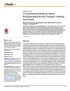
3.2. Qualitative assessment: SW propagation fronts From figure 7A (top panels), B corresponding to 20% and 48% of strain, a good match between experimental and numerical z-component velocities can be observed (z-axis is directed upwards) at three different time points. As the SW front propagating to the right in the experiments was not captured well enough (most probably due to the generated side lobe) it is not used for the comparison. Both experimental and numerical fronts demonstrated similar downward velocities distribution and attenuation (colour-coded in red in Fig. 7 corresponds to the “negative” parts of the graphs in Fig. 7). Although, for 20% and 48% of strain at time point 𝑡3 experimental downward velocities seemed to attenuate faster. Abaqus mimicked well the broadness of experimental SW fronts. The fronts were also broader for 48% of strain (figure 7A) as compared to 20% of strain for both numerical and SWE results. The overall upward relaxation movement was captured well both in Abaqus and in the SWE results (colourcoded in blue and corresponds to centre regions of the “positive” parts of the graphs in Fig. 7). In the numerical results, trailing upward directed velocities (in Fig. 7A at the lowest panel and two side peaks on the “positive” parts of the graphs in Fig. 7A, top panel, and 7B) could be observed behind the main SW fronts, and prominent at 𝑡2 and 𝑡3 . These peaks are not visible in the experimental results. 3.3. 2D view of SW fronts: looking into anisotropy of the model Figure 8 shows the modelled SW physics for different US probe orientations in the top view of the model (at the depth of 2 mm) for 20% and 48% of strain at 𝑡1 = 0.35ms and 𝑡2 = 0.75ms. An ellipsoidal wave front is excited, more prolonged for the increasing strain along its major semi-axis and almost unaffected along the minor semiaxis. The shape of the ellipse is independent from the probe orientation. While in the nearfield (t < 0.1-0.14 ms) the distribution of the z-component velocities corresponded to the ARF angle, after the SW fronts started to evolve such dependence began to disappear. However, as the wave front further developed, the distribution of the tissue velocities looked rather uniform for the complete ellipse and identical for different ARF angles.


12

The fibre angles were equal to 11° for 20% of strain and 8° for 48% of strain (with unstressed value of 15°). No obvious indication of the influence of the fibre angles on the elliptical SW fronts development could be recognized. The angles were contributing more to the orthotropic response with increased strain, i.e. influencing the shape of the ellipse.

Figure 7. A: Top 3 panels: Normalized experimental and numerical z-component velocities derived in the centre of the tissue slab and model, plotted at 3 corresponding time points (𝑡1𝑁𝑢𝑚 = 0.07 𝑚𝑠, 𝑡1𝑆𝑊𝐸 = 0.35 𝑚𝑠; 𝑡2𝑁𝑢𝑚 = 0.29 𝑚𝑠, 𝑡2𝑆𝑊𝐸 = 0.55 𝑚𝑠; 𝑡3𝑁𝑢𝑚 = 0.44 𝑚𝑠, 𝑡3𝑆𝑊𝐸 = 0.75 𝑚𝑠) along the lateral distance at 20% of strain. Bottom rows panels: Normalized z-component velocities demonstrating SW fronts in the cross-section of the tissue slab and the model. B: Normalized experimental and numerical z-component velocities plotted at 3 corresponding time points (t1Num = 0.10 ms, t1SWE = 0.35 ms; t 2Num = 0.29 ms, t 2SWE = 0.55 ms; t 3Num = 0.43 ms, t 3SWE = 0.75 ms) at 48% of strain.


13

Figure 8. Numerical results of SWs propagation fronts in the top middle view of the model at the depth of 2mm are displayed at time points of 𝑡1 = 0.35 𝑚𝑠 and 𝑡1 = 0.75 𝑚𝑠 at strain levels of 20% (Panel A) and 48% (Panel B) for different ARF orientation angles (0°, 30°, 90°). Two families of fibres are shown with a grey solid line with an angle of 11° corresponding to 20% of strain and an angle of 8° corresponding to 48% of strain; US probe imaging plane (ARF application angle) is displayed with a black dashed line.

3.4. Quantitative assessment: Group speed results Numerical group speed results were calculated for 6 models. The results for models IV and VI with fibres angles of 15° and 38° can be found in figure 9 A, B. The polar angle on the plots indicates the ARF angle and each ellipse represents the SWS for every strain level of 20%, 26%, 37% and 48%. The FE models provided a good fit with the experimental SWS results demonstrating little differences for different fibres angles and dispersion coefficients. Average difference between maximum and minimum SWS values for six models was 5.6±4.5%. For further consideration and as R2 and RMSE criteria were not helpful to


14

select a single model, we chose the model IV with a fibre angle of 15° and dispersion parameter of 0.2 as it seemed to give the closest match to the experimental SWS results. For both the model IV and SWE results, the highest SWS variation (figure 9 A, C) was observed for 0/180° ARF m angles in the direction of stretch. The experimental SWS was 6. 65 ± 0.13 versus a numerical SWS of 6. 63 ± 0.02

m s

at 20% of strain and 10.46 ± 0.01

m s

versus 10.88 ± 0.76

m s

s

at 48% of strain respectively. Other

values for experimental and numerical SWS results SWS are given in figure 9 D.

Figure 9. A, B: Polar plots representing the dependence of the SWS (the radial coordinate) on the ARF angle at different strain levels for numerical models IV and VI with the fibre angle of 15° and 38° , respectively, and dispersion parameter 𝜅 = 0.2. C: Experimental SWS results. D: Numerical and experimental SWS values for different ARF angles and strain levels.

3.5. Phase velocity results based on 2D FFT In order to investigate the influence of stress and anisotropy on the dispersion curves, the phase velocity analysis was performed for 20% and 48% of strains at 0°, 30° and 90° ARF angles with the results depicted in figure 10. The main anti-symmetric mode A0 was clearly visible and is shown with a solid orange line. For 20% of strain 4 other higher-order modes and for 48% of strain 3 higher-frequency modes were identified for 0° ARF angle. For 90° ARF angle, at 20% and 48% of strain 5 higher-order modes were identified. For 0° ARF angle, the plateau 𝑐𝑝 value of the A0 wave mode tends to increase with increasing strain values. The levelling off fd-value also increases from ≈2.9 kHz*mm to ≈3.3 kHz*mm, indicating that the A0 mode is dispersing at broader fd-range for higher strain values. For 90° ARF angle, the plateau 𝑐𝑝 value remains constant across different strains and the fd-number shift is not observed. The maximum fd-number for this analysis is defined by the Nyquist criterion, where the shortest wavelength (i.e. the highest fd-number) has the size of two pixels on the SWS map. This means that the maximum temporal frequency 𝑓 depends on the time sampling and the maximum spatial frequency 𝑘 is related to the lateral spacing on the SWS map.


15

Figure 10. Dispersion curves derived based on the 2D FFT analysis of the SWS maps at 20% and 48% of strain levels for 0°, 30° and 90° ARF angles.

3.6. Phase velocity results based on extracted stretch values Solution of (10)-(11) for the range of temporal frequencies 𝑓 and phase velocities 𝑐𝑝 derives analytical dispersion curves. These equations are complex transcendental equations. Therefore, a numerical approach was adopted to solve them, where the right-hand side values were calculated for a fixed 𝑐𝑝 , plate thickness 𝑑, 𝐶0 matrix and frequency 𝑓. Lamb-wave equations for symmetric and anti-symmetric modes were solved for all the ARF angles for 20% and 48% of strain (figure 11). To provide the best match to the 2D FFT-based results, maximum values of split coefficients in the push-forward stiffness elasticity tensor were taken (more information in Appendix B). For 0° and 90° ARF angles horizontal shear (SH) and quasi-shear modes were decoupled, so SH were not present in these plots. For 30° and 60° ARF angles these modes were coupled, and SH modes were present in the 30° ARF angle plot (even though not separately indicated due to their irrelevance for this study). Like for the 2D FFTbased analysis, more higher-order modes (4) could be observed for 20% of strain as compared to 48% of strain (1) for 0° ARF angle, which for 90° ARF angle 6 modes were observed for 20% of strain versus 4 modes for 48% of strain. The results also showed that the levelling off 𝑐𝑝 value for the A0 mode was achieved at similar fd values as compared to the 2D FFT, even though with a steeper linear slope at lower fd values. For 20% of strain, analytically computed 𝑐𝑝 plateau values for 0°, 30°, 60° and 90° ARF angle were 6.2, 6.1, 5.3, 4.5 m/s respectively, as compared to 6.8, 6.0, 4.8 and 4.5 m/s based on the 2D FFT. For 48% of strain and 0° ARF angle, analytical 𝑐𝑝 plateau value was lower (10 m/s) than the 2D FFT-based result (11.1 m/s). The opposite was true for 30°, 60° and 90° ARF angles with 9.6, 8.1, 5.5m/s analytical results versus 7.6, 5.2 and 4.6 m/s 2D FFT-based results.


16

Figure 11. Dispersion curves derived based on solving Lamb wave type equations for symmetric (S) and antisymmetric (A) modes at 20% and 48% of strain levels for 0 °, 30° and 90° ARF angles.

3.7. Skew angle and the energy velocity The skew angles for the A0 mode at for 20% and 48% of strain are given in table 2. The fd value was equal to 5 kHz*mm in order to compare the plateau regions. The skew angles indicated that for 0° and 90° ARF angles the wave energy (group velocity) vector is parallel to the wave propagation direction, whereas for 30° and 60° ARF angles it was not. Using (13) we calculated the energy velocity 𝑐𝑒 values which are given in table 3. For 0° ARF angle and 20%/48% of strain, 𝑐𝑒 values were higher for 2D FFT-based results as compared to the analytical ones. For 90° ARF angle, 𝑐𝑒 for 2D FFT-based results did not change with different strain levels. For the analytical solution 𝑐𝑒 increased from 4.5 m/s to 5.5 m/s. Assuming 𝑐𝑒 equal to the group velocity 𝑐𝑔 in the lossless media, both 2D FFT-based and analytical 𝑐𝑔 values gave a good match to the previously derived SWS (section 3.4). For 0° ARF angle, the average difference (20%/48% of strain) between the SWS and the 2D FFT-based/analytical results was 4.4% and 5.4% respectively. For 90° ARF angle, a perfect match between the SWS and 2D FFT-based results was obtained, while it was 10% difference between the SWS and analytical results. For 30° and 60° ARF angles, higher differences between 2D FFT-based and SWS results were observed, giving 7.6% and 7.3% for respectively. Between analytical and SWS results 11.8% and 23.2% differences were observed respectively. Characteristic wave surfaces were created with the radial coordinate corresponding to 𝑐𝑒 , the polar coordinate corresponding to the sum of the ARF and skew angles (figure 12). A good match between 2D FFT-based and analytical wave surfaces can be seen, with the wave surfaces being elongated along the stretching direction (towards the 0° ARF angle).


17

Table 2. Skew angles for A0 mode at fd=5 kHz*mm, based on 2D FFT-based and analytical dispersion curves (negative angles are counted clockwise, positive – counter clockwise). ARF angle Model IV 0° 30° 60° 90° Skew angle for A0 mode 2D FFT 0.6° -23° -16° 0.3° Strain 20% Analytical 0.7° -13° -18° -0.5° 2D FFT -1.5° -17° -25° 0.45° Strain 48% Analytical 0° -20° -31° -0.9° Table 3. Energy velocity (group speed) results for A0 wave mode and fd = 5 kHz*mm. ARF angle Model IV 0° 30° 60° 90° SWS 6.6 6 4.8 4.5 Strain 20%

Strain 48%

Energy velocity for A0 mode, fd = 5 2D FFT Analytical

6.8 6.2

6.6 6.1

5 5.3

4.5 4.5

SWS

10.5

7.5

5.1

4.6

Energy velocity for A0 mode, fd = 5 2D FFT Analytical

11.1 10

8 9.6

5.7 8.1

4.6 5.5

Figure 12. Wave surface profiles for the A0 wave mode at fd values of 5 kHz*mm (corresponds to the plateau region of the dispersion curve, shown on top panels) derived at 20% (orange line) and 48% (green line) of strain levels by plotting 𝑐𝐸 versus 𝛼 + 𝜑 with 𝛼 denoting the ARF (wave propagation) angle and 𝜑 denoting the skew angle. A: 2D FFT-based dispersion curve was used; B: Analytically derived dispersion curve was used.

4. Discussion 4.1. Numerical model – agreement with experimental data We performed the numerical modelling of the SWs propagating in an orthotropic plate (thickness 4 mm) subjected to different levels of stress. We investigated the directional dependency of the SWs by changing the ARF angle to mimic the rotation of the US probe around its axis. We validated our numerical model against the experimental SWE results by replicating the BCs, loading and by fitting the measured mechanical stress-strain data to the orthotropic material law. Assessing the anisotropic architecture of arteries with SWE (Chu & Rutt, 1997; Woodrum et al., 2006; Fujikura et al., 2007; Bernal et al., 2011; Ramnarine et al., 2014; Shcherbakova et al., 2014; Widman et al., 2016) could support the diagnosis of early-stage collagen remodelling and atherosclerosis. The potential of SWE to detect tissue anisotropy was previously shown for in-vitro tissue phantoms (Chatelin et al., 2014; Aristizabal et al., 2014) for skeletal and cardiac muscle (Gennisson et al., 2010; Urban et al., 2016; Rudenko & Sarvazyan, 2006; Pernot et al., 2007) and kidneys (Amador et al., 2011). However, most of the studies in literature have mainly


18

focused on bulky transverse isotropic materials with only one family of fibres (Rudenko & Sarvazyan, 2006; Gennisson et al., 2010; Royer et al., 2011; Rudenko & Sarvazyan, 2014; Chatelin et al., 2015; Urban et al., 2016; Guo et al., 2015; Chatelin et al., 2014). Arterial layers consist of (minimally) two families of collagen fibres with different orientations which lends them an orthotropic and nonlinear response. In this work we tried to overcome the limitations of the current literature, using the nonlinear orthotropic HGO material law to describe the mechanical behaviour of arterial tissue. The derived correction factors for six models (for different collagen fibre dispersion parameters and angles), indicated that the stresses in the SWE measurements region were 52-62% higher than the stresses derived from the mechanical measurements. This may also explain the differences found in our experimental results [7], where the incremental elastic modulus derived from the SWE in the direction of stretch (circumferential direction) was 50 to 56% higher than the one derived from the mechanical data. A good match between experimental and numerical SWS results was observed for all the models I-VI. While little differences were observed between the numerical models themselves – despite different fibre angles (15°, 30° and 38°) and dispersion parameters (0.1, 0.2) – model IV provided the best match with the experimental SWS results. For all the models and 0° ARF angle numerical SWS values replicated accurately the experimental results, while for 90° ARF angle SWS values demonstrated the largest difference (1.8 m/s or 37% for model VI at 48% of strain). This could probably be explained by the fact that the material law was fitted to the uniaxial data in the circumferential direction corresponding to 0° ARF angle. The material response at 90° ARF angle was not known. The observed little differences in SWS between all six numerical models could be due to the fact that we selected 𝜅 and fibre angles, while the rest of the coefficients 𝜇, 𝑘1 , 𝑘2 were obtained based on the best fit to the same experimental stress-strain data. Moreover, under different applied strain levels varying from 20 to 48%, the modelled collagen fibres elongated towards the stretching direction, changing from 30° to 16° (models I-II), 15° to 8° (models III-IV), from 38° to 21° (models V-VI). Hence, with increasing stretch, the fibres became more aligned. This indicates that SWS results are influenced by the overall orthotropic state of the material and the amount of stress inside the tissue, but not the collagen fibres themselves. Moreover, our simulations demonstrated that this effect is not related to different ARF angles. The structure in the 2D SW front ellipse developed at later times and was generated from the anisotropy and stretching of the model. The higher the level of strain, the more prolonged the ellipse was along its major semi-axis, confirming the increased stiffness of the material in this direction. Additionally, higher stress levels lead to a wider SW front in the direction of stretch (figure 8B and 9B), which could potentially indicate the need of higher frame rates to avoid merging of the SW fronts in time. A directional dependence of the SWS induced by the orthotropic nature of the material and its nonlinearity demonstrates that the imaging plane angle might be critical when imaging along or across collagen fibres to obtain consistent results. Especially at higher strain levels, SWS results will change more prominently depending on the imaging plane angle. Numerical and experimental results showed a close match between the SWs fronts propagating away from the excitation region, while the tissue velocity magnitude decreased faster in the experiment (figure 7A). This could be caused by the attenuation of the SW in the tissue due to the energy dissipation (Rudenko & Sarvazyan, 2014; Bercoff et al., 2004b). Additionally, almost no relaxation movement was observed (figure 8A) in the SWE results (most likely due to the low signal to noise ratio), whereas it was more prominent in the numerical results. Phase analysis was performed based on a 2D FFT of the SWS map in order to obtain dispersion curves and identify propagating wave modes. Because 2D FFT treats an image as part of a periodically replicated array, edge effects between the neighbours of such arrays created high-frequency noise in the 2D spectrum (shown prominently at the bottom of the dispersion plots in figure 10), although such noise did not seem to influence the A0 mode and could be reduced by applying a window function. We also found that the amount of dispersion


19

(linear dependency of the phase velocity on frequency) observed in the frequency-phase velocity spectrum not only depended on the nature of the SWs but also on the size of the selected region on the SWS map. The smaller the selected region, the more dispersion was present at lower frequencies for the main energy A0 mode with a steeper slope of the linear region between the phase velocity and fd values. A0 mode’s levelling off also shifted to higher fd-values and the 𝑐𝑝 plateau value increased if less of the front was selected. While numerically we could rely on the whole SW front, experimentally our dispersion curves demonstrated such “viscoelastic” behaviour. However, when taking the same lateral distance – observational time region on the corresponding numerical SWS maps, numerical dispersion curves matched well experimental ones demonstrating similar “viscoelastic” behaviour, which was not implemented in the model. Hence, experimental dispersion curves were not considered due to these limitations. When performing 2D FFT on experimental results, such influence should be taking into account. Especially in the settings such as arteries, where sometimes it is challenging to obtain full propagating fronts (e.g. in the cross-sectional view). Based on the 2D FFT results derived from the idealized SW propagation conditions of the numerical model, we were still limited to the anti-symmetric A0 Lamb-wave mode. It was partially due to the waves’ excitation load applied perpendicularly to the plate. Although differentiating higher-order modes on the 2D FFT-based dispersion plots did not seem feasible (especially if smaller region of the SW front was used). Therefore, based on 2D FFT, the SW modes analysis was limited only to the A0 mode. Consistent with the SWS analysis, the plateau value of the phase velocity dispersion curve for the A0 mode was sensitive to the orthotropy and nonlinearity of the material, with higher stiffness indicating higher plateau values along 0° and 30° US probe angles (Figure 10). We observed much less dependency for 60° and 90° US probe angles, probably because no significant stiffening of the material occurred in these directions. Similar dependency of phase velocity dispersion curves with applied hydrostatic pressure was experimentally reported in porcine carotid arteries (Widman et al., 2016). 4.2. Analytical analysis – correspondence with numerical results Analytical studies of SW propagation in stressed bulk linear elastic media (Gennisson et al., 2008; Destrade et al., 2010b; Abiza et al., 2012) or general anisotropic/transverse isotropic bulk media (Destrade et al., 2010a; Cheviakov & Ganghoffer, 2015; Shams et al., 2011) were previously performed. These studies did not focus on the SW propagation within restricting boundaries of the plate and considering the orthotropic material. Hence, the SWs physics were investigated within these settings. In addition, as arteries are nonlinear, the influence of stress on the material response and subsequently, on SWs was taken into account. It was done by obtaining the elasticity matrix not only dependent on the material properties, but also on the amount of the applied stress. Even though a commercial tool such as Disperse software (Pavlakovic et al., 1997) is available to generate dispersion curves for anisotropic materials, it only works for stress-free cases. Analytically describing and solving the case of the orthotropic material subjected to stress is challenging due to the splitting of the effective elastic constants in the push-forward elasticity tensor. Another approach in the theory of acoustoelasticity could be using third-order elastic constants (Duquennoy et al., 2008; Destrade et al., 2010b), but such constants were not available for our tissue and are difficult to measure. While deriving the elasticity matrix for 0° and 90° ARF angles at specific levels of stretch, 9 effective elastic constants were necessary to describe the material behaviour. However, for 30° or 60° ARF angles 13 effective elastic constants had to be defined, increasing the order of anisotropy in the presence of stress with respect to the SW propagation direction. This was caused due to the coupling between quasi-shear and horizontal shear modes for 30° and 60° ARF angles. For 0° and 90° ARF directions splitting between these shear modes was present. Despite this, the splitting was not visually seen on the SW propagation plots in figure 9, as similarly reported in case of the transverse isotropic material (Rouze et al., 2013), probably due to quasi-shear and horizontal shear velocities being quite similar to each other. While the 2D FFT-based approach could not provide with the information about higher-order wave modes present, phase curves derived from solving wave equations for symmetric and anti-symmetric A0 modes gave a


20

close match with the 2D FFT results. Although analytically calculated A0 mode plateau 𝑐𝑝 value for 0° ARF angle at 48% of strain was slightly lower than the one obtained from the 2D FFT, similar increase of 𝑐𝑝 with the higher levels of strain was observed for 0° and 30° US probe angles (along the stretch), while much less variation was present for 60° and 90° (across the stretch). For 0°/90° ARF angles and the A0 mode, we obtained the skew angles equal to 0°, i.e. phase velocities were equal to the energy (group) velocities (considering nonviscous media). These energy (group) velocity results from the plateau region of the A0 mode indicated a very good match with the time-of-flight SWS results for 0° or 90° ARF angles. Hence, when measuring along or across the collagen fibres, the plateau phase velocity A0mode value could be potentially equal to the time-of-flight SWS. This indicates that SWS is a collective parameter characterizing A0-mode propagation in these directions, while other modes are not contributing much to its value. For 30° or 60° ARF angles, significant skew angles indicated that the phase velocity and group velocity results were not equal. As for 30° or 60° ARF angles wave physics become more complicated (modes coupling, nonzero skew angles), it contributes to larger differences between the group speed results derived from the SWS and 2D FFT/analytical methods. 4.3. Limitations The HGO material model describes hyperelastic orthotropic material with two families of collagen fibres. As the material law is orthotropic, fitting to biaxial data is preferred over fitting to uniaxial data. Moreover, fibre angles and the dispersion parameter could not be derived experimentally and were assumed. Due to the sample’s geometry, overhanging of the tissue was present in the experiments, hence the stresses distribution was not homogeneous and the formula converting the mechanically measured force to the engineering/true stresses was not valid. Hence, the stresses measured with the mechanical testing machine and the stresses present in the SWE measurement region were significantly different (≈50%) and the conversion ratio between these stresses had to be calculated numerically. As observed in our experiments, the acoustic absorption affects the propagation of waves and causes the magnitudes of the z-component velocities to decrease in a real tissue. This effect was not included in the simulations and neither was the effect of viscoelasticity present in arteries. Experimental data is based on measurements on excised equine aortic tissue. While the microstructural organization and associated anisotropic behaviour of the tissue is similar as in humans, the thickness of the aortic wall will be much lower in humans. As such, caution is warranted when translating our findings to the human setting.

5. Conclusions The developed numerical model can be a useful tool for investigating shear wave propagation in orthotropic confined tissues such as arteries. This model demonstrated the importance of understanding and studying the shear wave propagation in stressed complex geometries subjected to realistic boundary conditions. In particular, group velocity analysis showed that shear wave speed was sensitive to the tissue’s orthotropy and nonlinearity, hence it was dependent on a specific measurement plane towards the collagen fibres/stretching direction. On the other hand, different acoustic radiation force angles did not influence the 2D shape and velocities distribution of the propagating shear fronts. Phase velocity analysis was more complex to perform due to the presence of different wave modes and complex equations describing wave propagation in the orthotropic material. While measuring along or across the stretching direction (in the circumferential or axial vessel’s planes) would give splitting of the quasi-shear and horizontal shear waves, measuring at other angles towards the stretching (e.g. 30° and 60° ARF angles) would give more complex results with coupling of the modes. Moreover, in the circumferential or axial vessel’s direction skew angles were found to be equal to 0°, indicating that the energy velocity and the wave propagation


21

directions were the same. In this case, for a particular wave mode and “frequency-plate thickness” number, the group velocity was equal to the energy velocity. In phase curve’s plateau regions, it also provided with a very good match to the shear wave speed values measured using a time-of-flight algorithm. For 30° and 60° ARF angles the number of independent elastic constants increased from 9 to 13 in the elasticity tensor, thus potentially challenging the inverse problem if that would be considered. As a result of more complex nature of the phase analysis, higher skew angles and higher differences between group velocities estimated based on the phase dispersion curves and time-of-flight algorithm were observed.

6. Acknowledgement Darya Shcherbakova is Ph.D. Fellow of the Research Foundation-Flanders (FWO-Vlaanderen), grant number 11U2116N. Abigail Swillens is Postdoctoral Fellow of the Research Foundation-Flanders (FWO-Vlaanderen), grant number 1276416N. Annette Caenen is Ph.D. Fellow of the IWT, grant number 141010. The authors gratefully acknowledge the financial support of the CWO, Faculty of Engineering and Architecture, Ghent University.


22

Appendix A: It is possible to calculate dispersion curves from the consideration of a stressed orthotropic material model and imposition of small perturbations created by propagating SWs on top of the stressed state. However, in order to consider incremental motions in a homogeneous medium subjected to homogeneous deformation and solve the equation of elastodynamics, the elasticity matrix for the stressed state must be known. Its derivation is given here for the Holzapfel-Gasser-Ogden model and based on (Gasser et al., 2006). The stressed state of the material is considered corresponding to specific strain values of the model. As arteries have nearly incompressible behaviour, the elastic response of the arteries can be split into the volumetric and isochoric parts. Then, the volume-independent deformation gradient F ′ can be calculated from the deformation gradient F and stretches λ1 , λ2 , λ3 in x,y,z – directions: 1

𝐹 ′ = 𝐽−3 𝐹

(A. 1)

The left Cauchy-Green stretch tensor associated with F ′ is given by 𝑏 ′ = 𝐹 ′ (𝐹 ′ )𝑇

(A. 2)

Fibres are assumed to be embedded in a continuum with their initial orientation characterized by unit vectors a 0 with index i denoting a fibres family: 𝑎0 𝑖 = [cos θ sin θ 0]

(A. 3)

The deformation of the fibres into their current stressed configuration can be represented by a vector a′ as: 𝑎𝑖 ′ = 𝐹 ′ 𝑎0 𝑖

(A.4)

Then, the fibres structure tensor depending of the orientation of the ith family of fibres 𝑎𝑖′ and dispersion parameters 𝜅 can be defined: ℎ𝑖′ = 𝜅𝑏 ′ + (1 − 3𝜅)(𝑎𝑖 ′ ⨂ 𝑎𝑖 ′ )

(A.5)

From that structure strain invariants can be calculated: 𝐸𝑖′ = 𝑡𝑟ℎ𝑖′ − 1

(A.6)

And stress and elasticity functions: 2

2

2

′ ′′ 𝜓𝑓𝑖 = 𝑘1 𝐸𝑖′ exp(𝑘2 𝐸𝑖′ ) , 𝜓𝑓𝑖 = 𝑘1 (1 + 2𝑘2 𝐸𝑖′ ) exp(𝑘2 𝐸𝑖′ ),

(A.7)

Isochoric Kirchhoff stress tensor: ′ ′ 𝜏̃ = 𝜏̃𝑔 + ∑2𝑖=1 𝜏̃𝑓𝑖 , 𝜏̃𝑔 = 𝐶10 𝑏 ′ , 𝜏̃𝑓𝑖 = 2𝜓𝑓𝑖 ℎ𝑖 1

𝜏 ′ = Ρ: 𝜏̃ , Ρ = ΙΙ − 𝐼⨂𝐼

(A.8) (A.9)

3

The isochoric spatial elastic tensor can then be defined from the stresses calculated above as: 2

2

3

3

4

′′ (𝑃: ℎ𝑖′ )⨂(𝑃: ℎ𝑖′ ) 𝐶 ′ = 𝑡𝑟(𝜏̃ )𝑃 − (𝜏 ′ ⨂𝐼 + 𝐼⨂𝜏 ′ ) + 4𝐽−3 ∑2𝑖=1 𝜓𝑓𝑖

(A.10)

Volume-dependent elastic tensor based on the assumption of the small compressibility in Abaqus will be defined as:

ARTERIAL SHEAR WAVE ELASTOGRAPHY MODELLING 𝐶𝑣𝑜𝑙 = (𝐽

𝜕𝜓 𝜕𝐽

+ 𝐽2

𝜕2 𝜓 𝜕𝐽2

) 𝛿⨂𝛿 − 2𝐽

𝜕𝜓 𝜕𝐽

II

23 (A.11)

Where 𝛿 is Dirac delta function. Then total stiffness can be defined as a sum of volume-independent and volume-dependent stiffness parts: 𝐶𝑡𝑜𝑡 = 𝐶 ′ + 𝐶𝑣𝑜𝑙

(A.12)

In order to consider incremental motions in a homogeneous medium subjected to homogeneous deformation, equation of elastodynamics for anisotropic compressible medium is (Ogden, 2015): 𝜌

𝜕2 𝑢 𝜕𝑡 2

= 𝐶0 𝑖𝑗𝑘𝑙

𝜕 2 𝑢𝑙 𝜕𝑥𝑖 𝜕𝑥𝑘

(A.13)

Where 𝐶0 is a Eulerian elasticity tensor (push-forward) of the stiffness matrix 𝐶𝑡𝑜𝑡 and defined as: 𝐶0𝑝𝑖𝑞𝑗 = 𝐽−1 𝐹𝑝𝛼 𝐹𝑞𝛽 𝐶𝛼𝑖𝛽𝑗 and 𝑢 is a small dynamic displacement which is superposed upon the initial finite static deformation.

(A.14)


24

Appendix B: Three deformation states had to be considered to describe wave propagation in a stressed state of the model. The first deformation state, called the natural state, describes the unstressed configuration and was defined in the 𝑥 0 , 𝑦 0 , 𝑧 0 coordinate system. The second deformation state, called the initial state, considers the applied uniaxial stress, i.e. deformed model at different strain levels and was defined in 𝑥, 𝑦, 𝑧 coordinate system. The final state accounts for the dynamic perturbation caused by the wave propagation, that is superimposed on the initial (stressed) state and was defined in x1 , x2 , x3 coordinate system. We were interested in investigating and studying our model behaviour in that final state in order to derive the wave propagation for different ARF angles and strain levels (Cheviakov & Ganghoffer, 2015; Shams et al., 2011; Ogden & Singh, 2014). Then in order to derive the wave equation for a stressed orthotropic plate, the governing equation of elastodynamics was solved in the final perturbation state (10). The push-forward elasticity matrix 𝐶0𝑖𝑗𝑘𝑙 with effective elastic constants was derived based on the HGO material coefficients and calculated stretches at every specific strain level. Its derivation is described in the Appendix A. Specific BCs corresponding to a plate in vacuum were taken into account, considering zero traction at plate’s boundaries. Due to the orthotropy of the material, no pure wave modes can be present in the tissue. Instead quasilongitudinal and quasi-shear modes will be generated. As quasi-longitudinal modes usually have much faster propagation speed, we did not consider them. Quasi-shear modes in plates are represented by symmetric and anti-symmetric Lamb waves. Symmetric Lamb wave modes can be classified into quasi-extensional (when the polarization vector is directed along the propagation direction) and quasi-horizontal shear (SH) modes (when the polarization vector is parallel to the plane of the plate). Anti-symmetric Lamb wave modes can be classified into the quasi-flexural and quasi-horizontal shear (SH) modes (Wang & Yuan, 2007; Rose, 2014). As the wave propagation in anisotropic plates depends on the direction of the propagation (Rose, 2014), decoupling of quasiextensional/quasi-flexural and SH type of wave equations for certain angles of propagation occurs. For these angles (0° and 90°) we only considered quasi-extensional and quasi-flexural wave modes, as these modes are the ones that are observed in the ultrasound imaging plane. For other angles (30° and 60°), coupling of symmetric Lamb modes and anti-symmetric Lamb modes occurs, hence separation of quasi-extensional/quasi-horizontal shear and quasi-flexural/quasi-horizontal shear modes was not possible analytically. a) ARF angles of 0° and 90° The canonical forms for the wave equations in the orthotropic stressed material for the Lamb waves propagating at the angles of 0° and 90° with displacements in the sagittal plane (x 1-x3) of the plate is derived from (10) and (11) : For symmetric Lamb modes: D11 D23 cot(γα1 ) − D13 D21 cot(γα3 ) = 0 











For anti-symmetric Lamb modes: D11 D23 tan(γα1 ) − D13 D21 tan(γα3 ) = 0 where γ =

2π𝑓 𝑐𝑝

(B.2)

h

∙ is the coefficient relating temporal frequency 𝑓, phase velocity 𝑐𝑝 and the plate thickness h. 2

These equations (B.1)-(B.2) and coefficients D11 , D13 , D21 , D23 come from the consideration of the boundary conditions (11) of the plate, expressed in terms of the partial wave displacements (Rose, 2014), and will have the form: D11 = C13 + α1 C33 W1 D13 = C13 + α3 C33 W3 D21 = α1 C55 + C55 W1 D23 = α3 C55 + C55 W3

(B.3)


25

with α1,3 being the roots of the acoustic tensor 𝐴, which are the functions of material properties and phase velocity 𝑐𝑝 : det 𝐴(𝛼) = 0

(B.4)

Generally, there will be six roots of α, however α1 = − α2 , α3 = − α4 , α5 = − α6 leading to symmetries in D and W coefficients, so we can exclude α2,4,6 from the equations. The components of 𝐴(𝛼) defined in a general form for an anisotropic material (triclinic symmetry) (Rose, 2014) as: 𝐴11 = 𝐶11 + 2𝐶15 𝛼 + 𝐶55 𝛼 2 − 𝜌𝑐𝑝 2 𝐴12 = 𝐶16 + (𝐶14 + 𝐶56 )𝛼 + 𝐶45 𝛼 2 𝐴13 = 𝐶15 + (𝐶13 + 𝐶55 )𝛼 + 𝐶35 𝛼 2

(B.5)

𝐴22 = 𝐶66 + 2𝐶46 𝛼 + 𝐶44 𝛼 2 − 𝜌𝑐𝑝 2 𝐴23 = 𝐶56 + (𝐶36 + 𝐶45 )𝛼 + 𝐶34 𝛼 2 𝐴33 = 𝐶55 + 2𝐶35 𝛼 + 𝐶33 𝛼 2 − 𝜌𝑐𝑝 2 Coefficients W1,3 represent the ratio between the wave displacement amplitudes in the sagittal plane 𝑈1 (𝛼) ⁄𝑈 (𝛼) found from solving the Christoffel’s equation (Rose, 2014): 3 𝐴𝑚𝑛 (𝛼)𝑈𝑛 = 0

(B.6)

If all of the terms of the matrix 𝐴 exist, the displacements in the three directions 𝑢1 , 𝑢2 , 𝑢3 are coupled together. However, for the case of 0° or 90° wave propagation, coefficients 𝐴12 and 𝐴23 are equal to 0 (which becomes obvious from the stiffness tensor coefficients and will not necessarily hold true for other propagation directions). Therefore, for this case the displacement ratios W1,3 will be reduced to the following form: W1,3 =

−A13 (α1,3 ) ⁄ A33(α1,3 )

(B.7)

The previously used coefficients 𝑈1 and 𝑈3 are the 𝑥1 - and 𝑥3 - components of the wave’s displacement amplitudes. The displacements themselves 𝑢1 , 𝑢2 , 𝑢3 are defined using the partial wave technique (Auld, 1990; Rose, 2014) by means of a harmonic exponential to describe the wave behaviour in the wave propagating direction along 𝑥1 -axis within confined boundaries of a plate in the form, with k representing the wave number, 𝑡 is time and 𝛼 is the coefficient linking displacements in the 𝑥3 -direction to 𝑥1 -direction: 𝑢1 = 𝑈1 𝑒 −𝑖𝑘(𝑥1 +𝛼𝑥3 −𝑐𝑝 𝑡) 𝑢2 = 𝑈2 𝑒 −𝑖𝑘(𝑥1 +𝛼𝑥3−𝑐𝑝𝑡)

(B.8)

𝑢3 = 𝑈3 𝑒 −𝑖𝑘(𝑥1 +𝛼𝑥3−𝑐𝑝𝑡) Coefficients 𝐶𝑖𝑗 are the coefficients of the push-forward stiffness tensor. In case of the wave propagating at 0° or 90° towards the direction of applied stretch, the push-forward stiffness matrix will have the form:

ARTERIAL SHEAR WAVE ELASTOGRAPHY MODELLING 𝐶11 𝐶12 𝐶13 𝐶21 𝐶22 𝐶23 𝐶 𝐶32 𝐶33 𝑪′ = 31 0 0 0 0 0 0 [ 0 0 0

0 0 0

𝐶44 0 0

0 0 0 0 0 0 0 0 𝐶55 0 0 𝐶66 ]

26

(B.9)

In this matrix 𝐶44 , 𝐶55 , 𝐶66 are split coefficients, meaning that more than one value of these coefficients can exist in the push-forward stiffness tensor, where the classic symmetry of second-order elastic tensor 𝐶𝑖𝑗𝑘𝑙 = 𝐶𝑗𝑖𝑙𝑘 = 𝐶𝑗𝑖𝑘𝑙 = 𝐶𝑖𝑗𝑙𝑘 does not hold and the contracted notation can have more than one value. The splits appear due to the consideration of the applied stress in the elastic tensor, where we are considering the stressed model as an unstressed with effective elastic constants (EEC) in the 𝑪′ matrix taking into account the stresses (Hughes & Kelly, 1953; Duquennoy et al., 2008). Therefore, by defining the 𝑪′ matrix we translate the dependence of the wave propagation velocity in relation to the field of stress in equation (B.10). Moreover, as the material properties in the 90° (axial) direction will be different from the material properties in the direction of stretch (0° circumferential direction), the material 𝑥, 𝑦, 𝑧 coordinate system will have to be rotated 90°. The derivation of the wave equations (B.1)-(B.2) and the form of the stiffness matrix (B.9) will stay the same for 90° wave propagation as it is for 0° and the stiffness matrix transformation will have to be performed: ′ 𝐶 ′′ 𝑚𝑛𝑜𝑝 = 𝛽𝑚𝑖 𝛽𝑛𝑗 𝛽𝑜𝑘 𝛽𝑝𝑙 𝐶𝑖𝑗𝑘𝑙

(B.10)

Where 𝛽 is a rotation matrix which is defined as: cos γ sin γ 𝛽 = [−sin γ cos γ 0 0

0 0] 1

(B.11)

with γ being the angle of wave propagation towards the stretching direction. b) ARF angles of 30° and 60° For the waves propagating at the angles of 30° and 60° all the terms of the 𝐴 matrix exist (B.5), therefore no decoupling between horizontal shear and Lamb-type waves occur. Therefore, instead of getting a pure longitudinal or pure SW we obtain quasi-longitudinal and quasi-shear partial waves. The canonical equations describing the Lamb modes become more complex: For symmetric Lamb modes: D11 G1 cot(γα1 ) + D13 G3 cot(γα3 ) + D15 G5 cot(γα5 ) = 0

(B.12)

For anti-symmetric Lamb modes: D11 G1 tan(γα1 ) + D13 G3 tan(γα3 ) + D15 G5 tan(γα5 ) = 0

(B.13)

𝐺1 = 𝐷23 𝐷35 − 𝐷33 𝐷25 𝐺2 = 𝐷31 𝐷25 − 𝐷21 𝐷35

(B.14)

𝐺3 = 𝐷21 𝐷33 − 𝐷31 𝐷23 D1(1,3,5) = C13 + α(1,3,5) C33 W(1,3,5) + C36 V(1,3,5) D2(1,3,5) = α(1,3,5) C55 + α(1,3,5) C45 V(1,6) + C55 W(1,3,5) D3(1,3,5) = α(1,3,5) C45 + α(1,3,5)1 C44 V(1,6) + C45 W(1,3,5)

(B.15)


27

The derivation of these equations is similar to the one described above, however, the displacements in the three 𝑈 (𝛼 ) directions 𝑢1 , 𝑢2 , 𝑢3 are coupled together and both displacement ratios W1,3,5 = 1 1,3,5 ⁄ and 𝑈3 (𝛼1,3,5 ) V1,3,5 =

𝑈2 (𝛼1,3,5 ) ⁄ will have the following form: 𝑈1 (𝛼1,3,5 ) W1,3,5 = V1,3,5 =

A13 (α1,3,5 )A12 (α1,3,5 )−A11 (α1,3,5 )A23 (α1,3,5 ) A23 (α1,3,5 )A13 (α1,3,5 )−A33 (α1,3,5 )A12 (α1,3,5 )

A11 (α1,3,5 )A23 (α1,3,5 )−A12 (α1,3,5 )A13 (α1,3,5 ) A13 (α1,3,5 )A22 (α1,3,5 )−A12 (α1,3,5 )A23 (α1,3,5 )

(B.16) (B.17)

For the wave propagation at 30°, 60° towards the direction of applied stretch, the stiffness matrix first has to be rotated according to the formulas (B.10)-(B.11) and the stiffness matrix will have to following form C11 C21 C31 C ′′ = 0 0 [C61

C12 C13 C22 C23 C32 C33 0 0 0 0 C62 C63

0 0 0 C44 C54 0

0 C16 0 C26 0 C36 C45 0 C55 0 0 C66 ]

(B.18)

As 𝐶44 , 𝐶55 , 𝐶66 were split coefficients in the 𝑪′ matrix before rotation transformation, after the rotation additional coefficients 𝐶61 , 𝐶62 , 𝐶63 , 𝐶16 , 𝐶26 , 𝐶36 , 𝐶45 , 𝐶54 in 𝑪′′ also become split. However, by selecting one of the split values for 𝐶44 , 𝐶55 , 𝐶66 in the 𝑪′ does not lead to additional splits for 𝐶61 , 𝐶62 , 𝐶63 , 𝐶16 , 𝐶26 , 𝐶36 , 𝐶45 , 𝐶54 in 𝑪′′ after the transformation.


28

7. REFERENCES Abiza, Z., Destrade, M., Ogden, R.W., Bordeaux, D., Albert, D. & Cedex, T. (2012). Large acoustoelastic effect. Wave Motion. 49. p.pp. 364–374. Alleyne, D.N. & Cawley, P. (1992). Optimization of lamb wave inspection techniques. NDT & E International. 25 (1). p.pp. 11–22. Amador, C., Member, S., Urban, M.W., Chen, S., Greenleaf, J.F. & Fellow, L. (2011). Shearwave Dispersion Ultrasound Vibrometry (SDUV) on Swine Kidney. IEEE Transactions on Ultrasonics, Ferroelectrics and Frequency Control. 58 (12). p.pp. 2608–2619. Dassault Systèmes 2012 ABAQUS Theory Manual, version 6.12 (Providence, RI, USA: Dassault Systèmes Simulia Corp.) Aristizabal, S., Amador, C., Qiang, B., Kinnick, R.R., Nenadic, I.Z., Greenleaf, J.F. & Urban, M.W. (2014). Shear wave vibrometry evaluation in transverse isotropic tissue mimicking phantoms and skeletal muscle. Physics in Medicine & Biology. 59. p.pp. 7735–7752. Auld, B.A. (1990). Acoustic fields and waves in solids. 2nd Ed. the University of California: R.E. Krieger (Malabar, FL: The University of California), 1990. Bercoff, J., Fink, M. & Tanter, M. (2004a). Supersonic Shear Imaging : A New Technique for soft tissue elasticity mapping. IEEE Transactions on Ultrasonics, Ferroelectrics and Frequency Control. 51 (4). p.pp. 396–409. Bercoff, J., Tanter, M., Muller, M. & Fink, M. (2004b). The role of viscosity in the impulse diffraction field of elastic waves induced by the acoustic radiation force. IEEE transactions on ultrasonics, ferroelectrics, and frequency control. 51 (11). p.pp. 1523–36. Bernal, M., Nenadic, I., Urban, M.W. & Greenleaf, J.F. (2011). Material property estimation for tubes and arteries using ultrasound radiation force and analysis of propagating modes. Journal of Acoustical Society of America. 129 (3). p.pp. 1344–1354. Caenen, A., Shcherbakova, D., Verhegghe, B., Papadacci, C., Pernot, M., Segers, P. & Swillens, A. (2015). A Versatile and Experimentally Validated Finite Element Model to Assess the Accuracy of Shear Wave Elastography in a Bounded Viscoelastic Medium. 62 (3). Chatelin, S., Bernal, M., Deffieux, T., Papadacci, C., Flaud, P., Nahas, A., Boccara, C., Gennisson, J.-L., Tanter, M. & Pernot, M. (2014). Anisotropic polyvinyl alcohol hydrogel phantom for shear wave elastography in fibrous biological soft tissue: a multimodality characterization. Physics in Medicine & Biologyy. 59. p.pp. 6923–6940. Chatelin, S., Gennisson, J., Bernal, M., Tanter, M. & Pernot, M. (2015). Modelling the impulse diffraction field of shear waves in transverse isotropic viscoelastic medium. Physics in Medicine & Biology. 60. p.pp. 3639–3654. Cheviakov, A.F. & Ganghoffer, J. (2015). One-dimensional nonlinear elastodynamic models and their local conservation laws with applications to biological membranes. Journal of the Mechanical Behavior of Biomedical Materials. p.pp. 1–17. Chu, K.C. & Rutt, B.K. (1997). Polyvinyl Alcohol Cryogel: An Ideal Phantom Material for MR Studies of Arterial Flow and Elasticity. MRM. 37. p.pp. 314–319. Couade, M., Pernot, M., Prada, C., Messas, E., Emmerich, J., Bruneval, P., Criton, A., Fink, M. & Tanter, M. (2010). Quantitative assessment of arterial wall biomechanical properties using shear wave imaging. Ultrasound in medicine & biology. 36 (10). p.pp. 1662–76. Destrade, M., Gilchrist, M.D. & Ogden, R.W. (2010a). Third- and fourth-order elasticity of biological soft tissues. Journal of Acoustical Society of America. 127. p.pp. 1–11. Destrade, M., Gilchrist, M.D. & Saccomandi, G. (2010b). Third- and fourth-order constants of incompressible soft solids and and the acousto-elastic effect. Journal of Acoustical Society of America. 127. p.pp. 2759– 2763.


29

Doherty, J.R., Trahey, G.E., Nightingale, K.R. & Palmeri, M.L. (2013). Acoustic radiation force elasticity imaging in diagnostic ultrasound. IEEE transactions on ultrasonics, ferroelectrics, and frequency control. 60 (4). p.pp. 685–701. Duquennoy, M., Ouaftouh, M., Devos, D., Jenot, F. & Ourak, M. (2008). Effective elastic constants in acoustoelasticity. Applied Physics Letters. 92 (24). p.p. 244105. Fujikura, K., Luo, J., Gamarnik, V., Pernot, M., Fukumoto, R., Tilson, M.D. & Konofagou, E.E. (2007). A novel noninvasive technique for pulse-wave imaging and characterization of clinically-significant vascular mechanical properties in vivo. Ultrasonic Imaging. 29 (3). p.pp. 137–154. Gasser, T.C., Ogden, R.W. & Holzapfel, G.A. (2006). Hyperelastic modelling of arterial layers with distributed collagen fibre orientations. Journal of the Royal Society, Interface. 3. p.pp. 15–35. Gennisson, J.-L., Deffieux, T., Mace, E., Montaldo, G., Fink, M. & Tanter (2010). Viscoelastic and anisotropic mechanical properties of in vivo muscle tissue assessed by Supersonic Shear Imaging. Ultrasound in medicine & biology. 36 (5). p.pp. 789–801. Gennisson, J., Rénier, M., Catheline, S., Barrière, C., Bercoff, J., Tanter, M. & Fink, M. (2008). Acoustoelasticity in soft solids: Assessment of the nonlinear shear modulus with the acoustic radiation force. Journal of Acoustical Society Of America. 122 (6). p.pp. 3211–3219. Guo, J., Hirsch, S., Scheel, M., Braun, J. & Sack, I. (2015). Three-Parameter Shear Wave Inversion in MR Elastography of Incompressible Transverse Isotropic Media : Application to In Vivo Lower Leg Muscles. Magnetic resonance in medicine. 0. p.pp. 1–9. Haskett, D., Johnson, G., Zhou, A., Utzinger, U. & Vande Geest, J. (2010). Microstructural and biomechanical alterations of the human aorta as a function of age and location. Biomechanics and modeling in mechanobiology. 9 (6). p.pp. 725–36. Holzapfel, G.A. (2001). Biomechanics of soft tissue. In: J. Lemaitre (ed.). Handbook of Material Behavior Models, Three-Volume Set: Nonlinear Models and Properties. Academic Press, p. 1200. Holzapfel, G.A. (2006). Determination of material models for arterial walls from uniaxial extension tests and histological structure. Journal of theoretical biology. 238. p.pp. 290–302. Holzapfel, G.A. & Gasser, T.C. (2001). A viscoelastic model for fiber-reinforced composites at finite strains: Continuum basis, computational aspects and applications. Computer Methods in Applied Mechanics and Engineering. 190 (34). p.pp. 4379–4403. Hughes, D.S. & Kelly, J.L. (1953). Second-Order Elastic Deformations of Solids. Physical Review. 92 (5). p.pp. 1145–1150. Lee, K.H., Szajewski, B.A., Hah, Z., Parker, K.J. & Maniatty, A.M. (2012). Modeling shear waves through a viscoelastic medium induced by acoustic radiation force. International Journal for Numerical Methods in Biomedical Engineering. p.pp. 1–19. McGough, R.J. (2004). Rapid calculations of time-harmonic nearfield pressure produced by rectangular pistons. Journal of Acoustical Society of America. 115. p.pp. 1934–1941. Ogden, R.W. (2015). Nonlinear Elasticity with Application to Soft Fibre-reinforced Materials. In: Nonlinear mechanics of soft fibrous materials. pp. 1–48. Ogden, R.W. & Singh, B. (2014). The effect of rotation and initial stress on the propagation of waves in a transversely isotropic elastic solid. Wave Motion. 51 (7). p.pp. 1108–1126. Palmeri, M.L., Member, S., Sharma, A.C., Bouchard, R.R., Nightingale, R.W. & Nightingale, K.R. (2005). A Finite-Element Method Model of Soft Tissue Force. 52 (10). p.pp. 1699–1712. Pavlakovic, B., Lowe, M., Alleyne, D. & Cawley, P. (1997). Disperse: A general purpose program for creating dispersion curves. Review of Progress in Quantitative Nondestructive Evaluation. 16. p.pp. 185–192. Pernot, M., Fujikura, K., Fung-Kee-Fung, S.D. & Konofagou, E.E. (2007). ECG-gated, mechanical and electromechanical wave imaging of cardiovascular tissues in vivo. Ultrasound in medicine & biology. 33 (7). p.pp. 1075–85.


30

Ramnarine, K. V, Garrard, J.W., Kanber, B., Nduwayo, S., Hartshorne, T.C. & Robinson, T.G. (2014). Shear wave elastography imaging of carotid plaques: feasible, reproducible and of clinical potential. Cardiovascular ultrasound. 12. p.pp. 1–8. Robertson, A.M. & Watton, P.N. (2013). Mechanobiology of the Arterial Wall. In: S. Becker & A. Kuznetsov (eds.). Transport in Biological Media. Elsevier, pp. 275–347. Rose, J.L. (2014). Ultrasonic Guided Waves in Solid Media. 1st Ed. New York: Cambridge University Press. Rouze, N.C., Wang, M.H., Palmeri, M.L. & Nightingale, K.R. (2013). Finite element modeling of impulsive excitation and shear wave propagation in an incompressible, transversely isotropic medium. Journal of Biomechanics. 46 (16). p.pp. 2761–2768. Royer, D., Gennisson, J.-L., Deffieux, T. & Tanter, M. (2011). On the elasticity of transverse isotropic soft tissues ( L ). Journal of Acoustical Society of America. 129 (4). p.pp. 8–13. Rudenko, O. V. & Sarvazyan, A.P. (2014). Wave Anisotropy of Shear Viscosity and Elasticity. Acoustical Physics. 60 (6). p.pp. 710–718. Rudenko, O. V & Sarvazyan, A.P. (2006). Wave Biomechanics of the Skeletal Muscle. Acoustical Physics. 52 (6). p.pp. 720–732. Rudenko, O. V, Sarvazyan, A.P. & Emelianov, S.Y. (1996). Acoustic radiation force and streaming induced by focused nonlinear ultrasound in a dissipative medium. Journal of Acoustical Society of America. 99 (May 2013). p.pp. 2791–2798. Sandrin, L., Fourquet, B., Hasquenoph, J.-M., Yon, S., Fournier, C., Mal, F., Christidis, C., Ziol, M., Poulet, B., Kazemi, F., Beaugrand, M. & Palau, R. (2003). Transient elastography: a new noninvasive method for assessment of hepatic fibrosis. Ultrasound in Medicine & Biology. 29 (12). p.pp. 1705–1713. Sarvazyan, A.P., Skovoroda, A.R., Emelianov, S.Y., Fowlkes, J.B., Pipe, J.G., Adler, R.S., Buxton, R.B. & Carson, P.L. (1995). Biophysical Bases of Elasticity Imaging. Acoustical Imaging. 21. p.pp. 223–240. Sarvazyan, A.P., Urban, M.W. & Greenleaf, J.F. (2013). Acoustic waves in medical imaging and diagnostics. Ultrasound in medicine & biology. 39 (7). p.pp. 1133–46. Shams, M., Destrade, M. & Ogden, R.W. (2011). Initial stresses in elastic solids: Constitutive laws and acoustoelasticity. Wave motion. 48. p.pp. 552–567. Shcherbakova, D.A., Papadacci, C., Swillens, A., Caenen, A., Bock, S. De, Saey, V., Chiers, K., Tanter, M., Greenwald, S.E., Pernot, M. & Segers, P. (2014). Supersonic Shear Wave Imaging to Assess Arterial Nonlinear Behavior and Anisotropy: Proof of Principle via Ex Vivo Testing of the Horse Aorta. Advances in Mechanical Engineering. 2014. p.pp. 1–11. Shcherbakova, D., Papadacci, C., Swillens, A., Caenen, A., Saey, V., De Bock, S., Chiers, K., Pernot, M. & Segers, P. (2013). Supersonic Shear Wave Imaging to Assess Arterial Anisotropy: Ex-vivo Testing of the Horse Aorta. In: IEEE International Ultrasonics Symposium 2013. 2013, pp. 1–4. Taelman, L., Degroote, J., Swillens, A., Vierendeels, J. & Segers, P. (2014). Fluid – structure interaction simulation of pulse propagation in arteries: Numerical pitfalls and hemodynamic impact of a local stiffening. International Journal of Engineering Science. 77. p.pp. 1–13. Urban, M.W., Qiang, B., Song, P., Nenadic, I.Z., Chen, S. & Greenleaf, J.F. (2016). Investigation of the effects of myocardial anisotropy for shear wave elastography using impulsive force and harmonic vibration. Physics in Medicine & Biology. 61. p.pp. 365–382. Verhegghe, B. (n.d.). pyFormex home page. [Online]. Available from: http://www.nongnu.org/pyformex/. Wang, L. & Yuan, F. (2007). Group velocity and characteristic wave curves of Lamb waves in composites: Modeling and experiments. Composites Science and Technology. 67. p.pp. 1370–1384. Widman, E., Maksuti, E., Amador, C., Urban, M.W., Caidahl, K. & Larsson, M. (2016). Shear wave elastography quantifies stiffness in ex vivo porcine artery with stiffened arterial region. Ultrasound in Medicine and Biology. 42 (10). p.pp. 2423–2435. Woodrum, D.A., Romano, A.J., Lerman, A., Pandya, U.H., Brosh, D., Rossman, P.J., Lerman, L.O. & Ehman,


31

R.L. (2006). Vascular wall elasticity measurement by magnetic resonance imaging. Magnetic resonance in medicine. 56. p.pp. 593–600.

A finite element model to study the effect of tissue anisotropy on ... - Core

A finite element model to study the effect of tissue anisotropy on ... - Core

Suggest Documents

Study on Finite Element Model Updating in

FINITE ELEMENT MODEL TO STUDY CALCIUM ...

A Finite Element Study

Finite Element Analysis and Experimental Study on the Effect of

The importance of nonlinear tissue modelling in finite element ... - Core

A Finite Element Study On - IOSR Journals

A Finite Element Analysis Study

A convection model to explain anisotropy of the inner core

Finite Element Model to Study Calcium Distribution in ...

Finite Element Model to Study Calcium Diffusion in ... - Google Sites

Effect of Mesh Parameters in Finite Element Simulation of ... - Core

The Effect of Numerical Integration on the Finite Element ... - ispacs

A Finite Element Model Based on Discontinuous Galerkin Methods on ...

Application of a finite-element model to low-frequency sound ...

Why To Study Finite Element Analysis

modelling the effect of plastic anisotropy on springback of ... - Core

Finite Element Analysis to Study The Effects Of The Workpiece

A Bio-Realistic Finite Element Model to Evaluate the Effect of

A tridimensional finite element approach to model a tunnel with

A Finite Element Analysis of a Human Foot Model to Simulate ... - Core

A global finite-element shallow-water model

A Finite Element Model for Mixed

A Three-Dimensional Finite Element Model ...

a discrete element model to consider the effect of pore