A Framework for Clustering Massive-Domain Data ... - Semantic Scholar

A Framework for Clustering Massive-Domain Data Streams Charu C. Aggarwal IBM T. J. Watson Research Center 19 Skyline Drive, Hawthorne, NY, USA [email protected]

Abstract— In this paper, we will examine the problem of clustering massive domain data streams. Massive-domain data streams are those in which the number of possible domain values for each attribute are very large and cannot be easily tracked for clustering purposes. Some examples of such streams include IP-address streams, credit-card transaction streams, or streams of sales data over large numbers of items. In such cases, it is well known that even simple stream operations such as counting can be extremely difficult because of the difficulty in maintaining summary information over the different discrete values. The task of clustering is significantly more challenging in such cases, since the intermediate statistics for the different clusters cannot be maintained efficiently. In this paper, we propose a method for clustering massive-domain data streams with the use of sketches. We prove probabilistic results which show that a sketch-based clustering method can provide similar results to an infinitespace clustering algorithm with high probability. We present experimental results which validate these theoretical results, and show that it is possible to approximate the behavior of an infinitespace algorithm accurately.

I. I NTRODUCTION In recent years, new ways of collecting data have resulted in a need for applications which work effectively and efficiently with data streams. One important problem in the data stream domain is that of clustering. The clustering problem has been widely studied because of its applications to a wide variety of problems in customer-segmentation and target-marketing [10], [11], [17]. A broad overview of different clustering methods may be found in [12], [13]. The problem of clustering has also been studied in the context of data streams [1], [3], [14]. In this paper, we will examine the problem of massivedomain stream clustering. Massive-domains are those data domains in which the number of possible values for one or more attributes is very large. Examples of such domains are as follows: • In network applications, many attributes such as IPaddresses are drawn over millions of possibilities. In a multi-dimensional application, this problem is further magnified because of the multiplication of possibilities over different attributes. • Typical credit-card transactions can be drawn from a universe of millions of different possibilities depending upon the nature of the transactions. • Supermarket transactions are often drawn from a universe of millions of possibilities. In such cases, the deter-

mination of patterns which indicate different kinds of classification behavior may become infeasible from a space- and computational efficiency perspective. The problem of massive-domain clustering naturally occurs in the space of discrete attributes, whereas most of the known data stream clustering methods are designed on the space of continuous attributes. Furthermore, since we are solving the problem for the case of fast data streams, this restricts the computational approach which may be used for discriminatory analysis. Thus, this problem is significantly more difficult than the standard clustering problem in data streams. Spaceefficiency is a special concern in the case of data streams, because it is desirable to hold most of the data structures in main memory in order to maximize the processing rate of the underlying data. Smaller space requirements ensure that it may be possible to hold most of the intermediate data in fast caches, which can further improve the efficiency of the approach. Furthermore, it may often be desirable to implement stream clustering algorithms in a wide variety of space-constrained architectures such as mobile devices, sensor hardware, or cell processors. Such architectures present special challenges to the massive-domain case, if the underlying algorithms are not space-efficient. The problem of clustering can be extremely challenging from a space and time perspective in the massive-domain case. This is because one needs to retain the discriminatory characteristics of the most relevant clusters in the data. In the massive-domain case, this may entail storing the frequency statistics of a large number of possible attribute values. While this may be difficult to do explicitly, the problem is further intensified by the large volume of the data stream which prevents easy determination of the importance of different attributevalues. In this paper, we will propose a sketch-based approach in order to keep track of the intermediate statistics of the underlying clusters. These statistics are used in order to make approximate determinations of the assignment of data points to clusters. We provide probabilistic results which indicate that these approximations are sufficiently accurate to provide similar results to an infinite-space clustering algorithm with high probability. We also present experimental results which illustrate the high accuracy of the approximate assignments. This paper is organized as follows. The remainder of this section discusses related work on the stream clustering

problem. In the next section, we will propose a technique for massive-domain clustering of data streams. We provide a probabilistic analysis which shows that our sketch-based stream clustering method provides similar results to an infinitespace clustering algorithm with high probability. In section III, we discuss the experimental results. We show that the experimental behavior of the sketch-based clustering algorithm behaves in accordance with the presented theoretical results. Section IV contains the conclusions and summary. A. Related Work The problem of clustering has been widely studied in the database, statistical and pattern recognition communities [10], [12], [13], [11], [17]. Detailed surveys of clustering algorithms may be found in [12], [13]. In the database community, the major focus in designing clustering algorithms has been to reduce the number of passes required in order to perform the clustering. For example, the algorithms discussed in [10], [11], [17] focus on clustering the underlying data in one pass. Subsequently, the problem of clustering has also been studied in the data stream scenario. Computational efficiency is of special importance in the case of data streams, because of the large volume of the incoming data. A variety of methods for clustering data streams are proposed in [1], [9], [14]. The techniques in [9], [14] propose k-means techniques for stream clustering. A micro-clustering approach has been combined with a pyramidal time-frame concept [1] in order to provide the user with greater flexibility in querying stream clusters over different time horizons. Recently the technique has been extended to the case of high dimensional data with the use of a projected clustering approach [2]. Details on different kinds of stream clustering algorithms may be found in [4]. Recently the problem of stream clustering has also been extended to domains other than continuous attributes. Methods for clustering binary data streams were presented in [16]. Techniques for clustering categorical and text data streams may be found in [15] and [18] respectively. A recent technique [3] was designed to cluster both text and categorical data streams. This technique is useful in a wide variety of scenarios which require detailed over different time horizons. The method in [3] can be combined with the concept of pyramidal time-frame in order to enable such an analysis. None of the above mentioned techniques are useful for the case of massive-domain data streams. At attempt to generalize these algorithms to the massive-domain case results in excessive space requirements. Such space-requirements can cause additional challenges in implementing stream clustering algorithms across a variety of recent space-constrained devices such as mobile devices, cell processors or GPUs. The aim of this paper is significantly broaden the applicability of stream clustering algorithms to very massive-domain data streams in space-constrained scenarios. II. S KETCH - BASED C LUSTERING M ODEL Before presenting the clustering algorithm, we will introduce some notations and definitions. We assume that the

data stream D contains d-dimensional records denoted by X1 . . . XN . . .. The attributes of record Xi are denoted by (x1i . . . xdi ). It is assumed that the attribute value xki is drawn k from the unordered domain set Jk = {v1k . . . vM k }. We note that the value of M k denotes the domain size for the kth attribute. The value of M k can be very large, and may range in the order of millions or billions. From the point of view of a clustering application, this creates a number of challenges, since it is no longer possible to hold the cluster statistics in a space-limited scenario. Sketch based techniques [6], [7] are a natural method for compressing the counting information in the underlying data so that the broad characteristics of the dominant counts can be maintained in a space-efficient way. In this paper, we will apply the count-min sketch [7] to the problem of clustering massive-domain data streams. We will demonstrate a number of important theoretical and experimental results about the behavior of such an algorithm. In the count-min sketch, a hashing approach is utilized in order to keep track of the attribute-value statistics in the underlying data. We use w = ⌈ln(1/δ)⌉ pairwise independent hash functions, each of which map onto uniformly random integers in the range h = [0, e/ǫ], where e is the base of the natural logarithm. The data structure itself consists of a two dimensional array with w·h cells with a length of h and width of w. Each hash function corresponds to one of w 1-dimensional arrays with h cells each. In standard applications of the count-min sketch, the hash functions are used in order to update the counts of the different cells in this 2-dimensional data structure. For example, consider a 1dimensional data stream with elements drawn from a massive set of domain values. When a new element of the data stream is received, we apply each of the w hash functions to map onto a number in [0 . . . h − 1]. The count of each of the set of w cells is incremented by 1. In order to estimate the count of an item, we determine the set of w cells to which each of the w hash-functions map, and compute the minimum value among all these cells. Let ct be the true value of the count being estimated. We note that the estimated count is at least equal to ct , since we are dealing with non-negative counts only, and there may be an over-estimation because of collisions among hash cells. As it turns out, a probabilistic upper bound to the estimate may also be determined. It has been shown in [7], that for a data stream with T arrivals, the estimate is at most ct + ǫ · T with probability at least 1 − δ. In this paper, we will use the sketch-based approach in order to cluster massive-domain data streams. We will refer to the algorithm was the CSketch algorithm, since the algorithm clusters the data with the use of sketches. The CSketch algorithm uses the number of clusters k and the data stream D as input to the algorithm. The clustering algorithm is partition-based, and assigns incoming data points to the most similar cluster centroid. The frequency counts for the different attribute values in the cluster centroids are incremented with the use of the sketch table. These frequency counts can be maintained only approximately because of the massive domain size of the underlying attributes in the data stream. Similarity is measured

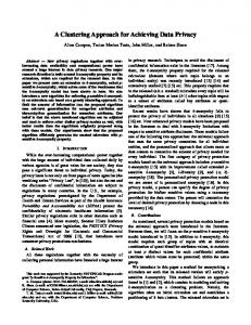
Algorithm CSketch(Labeled Data Stream: D, NumClusters: k) begin Create k sketch tables of size w · h each; Initialize k sketch tables to null counts; repeat Receive next data point X from D; Compute the approximate dot product of incoming data point with each cluster-centroid with the use of the sketch tables; Pick the centroid with the largest approximate dot product to incoming point; Increment the sketch counts in the chosen table for all d dimensional value strings; until(all points in D have been processed); end Fig. 1.

The Sketch-based Clustering Algorithm (CSketch Algorithm)

with the computation of the dot-product function between the incoming point and the centroid of the different clusters. This computation can be performed only approximately in the massive-domain case, since the frequency counts for the values in the different dimensions cannot be maintained explicitly. For each cluster, we maintain the frequency sketches of the records which are assigned to it. Specifically, for each cluster, the algorithm maintains a separate sketch table containing the counts of the values in the incoming records. It is important to note that the same hash function is used for each clusterspecific hash table. As we will see, this is useful in deriving some important theoretical properties of the CSketch algorithm. The algorithm starts off by initializing the counts in each sketch table to 0. Subsequently, for each incoming record, we will update the counts of each of the cluster-specific hash tables. In order to determine the assignments of data points to clusters, we need to compute the dot product of the ddimensional incoming records with the frequency statistics of the values in the different clusters. We note that this is not possible to do explicitly, since the precise frequency statistics are not maintained. Let qrj (xri ) represents the frequency of the value xri in the j-th cluster. Let mi be the number of data points assigned to the j-th cluster. Then, the d-dimensional statistics of the record (x1i . . . xdi ) for the j-th cluster is given by (q1j (x1i ) . . . qdj (xdi )). Then, the frequency-based dot-product Dj (Xi ) of the incoming record with statistics of cluster j is given by the dot product of the fractional frequencies (q1j (x1i )/mj . . . qdj (xdi )/mj ) of the attribute values (x1i . . . xdi ) with the frequencies of these same attribute values within record Xi . We note that the frequencies of the attribute values with the record Xi are unit values corresponding to (1, . . . 1). Therefore, the corresponding dot product is the following: Dj (Xi ) =

d X

qrj (xri )/mj

the estimated dot product is the largest. We note that the value of qrj (xri ) cannot be known exactly, but can only be estimated approximately because of the massive-domain constraint. There are two key steps which use the sketch table during the clustering process: • Updating the sketch-table and other required statistics for the corresponding cluster for each incoming record. • Comparing the similarity of the incoming record to the different clusters with the use of the corresponding sketch tables. First, we discuss the process of updating the sketch table, once a particular cluster has been identified for assignment. For each record, the sketch-table entries corresponding to the attribute values on the different dimensions are incremented. In some cases, the different dimensions may take on the same value when the values are drawn from the same domain. For example, in a network intrusion application, two of the dimensions may be source and destination IP-addresses. In such cases, we would like to distinguish between similar values across different dimensions for the purpose of statistics tracking in the sketch tables. A natural solution is to tag the dimension identification with the categorical value. Therefore, for the categorical value for each dimension r, we create a string which concatenates the following two values: r • The categorical value xi . • The index r of the dimension. We denote this string by xri ⊕ r. Therefore, each record Xi has a corresponding set of d strings which are denoted by x1i ⊕ 1 . . . xdi ⊕ d. For each incoming record Xi , we apply each of the w hash functions to the strings x1i ⊕ 1 . . . xdi ⊕ d. Let m be the index of the cluster to which the data point is assigned. Then, exactly d · w entries in the sketch table for cluster m are updated by applying the w hash functions to each of the d strings which are denoted by x1i ⊕ 1 . . . xdi ⊕ d. The corresponding entries are incremented by one unit each. In addition, we explicitly maintain the number of records mj in cluster j. Next, we discuss the process of comparing the different clusters for similarity to the incoming data point. In order to pick a cluster for assignment, the approximate dot-products across different clusters need to be computed. As in the previous case, the d strings x1i ⊕ 1 . . . xdi ⊕ d are constructed. Then, we apply the w hash functions to each of these d strings. We retrieve the corresponding d sketch-table entries for each of the w hash functions and each cluster. For each of the w hashfunctions for the sketch table for cluster j, the d counts are simply estimates of the value of q1j (x1i ) . . . qdj (xdi ). Specifically, let the count for the entry picked by the lth hash function corresponding to the rth dimension of record Xi in the sketch table for cluster j be denoted by cijlr . Then, we estimate the dot product Dij between the record Xi and the frequency statistics for cluster j as follows:

(1)

r=1

The incoming record is assigned to the cluster for which

Dij = minl

d X r=1

cijlr /mj

(2)

The value of Dij is computed over all clusters j, and the cluster with the largest dot product to the record Xi is picked for assignment. We note that the distribution of the data points across different clusters is not random, since it is affected by counts in the sketch table entries. Furthermore, since the process of incrementing the sketch tables depends upon cluster assignments, it follows that the distribution of counts across hash-table entries is not random either. Therefore, a direct application of the properties in [7] to each cluster-specific sketch table would not be valid. Furthermore, we are interested in preserving the ordering of the dot-products as opposed to the absolute values of the dot products. This ensures that the clustering assignments are not significantly affected by the approximation process. In the next section, we will provide an analysis of the effectiveness of using a sketch-based approach. A. Analysis We would like to determine the accuracy of the clustering approach, since we are using approximations from the sketch table in order to make key assignment decisions. In general, we would like the behavior of the clustering algorithm to mirror the behavior of an infinite-space algorithm as much as possible. While the dot product computation is approximate, it is really the ordering of the values of the different dot products that matters. As long as this ordering is preserved, the behavior of the clustering algorithm will be similar to that of an infinite-space algorithm. The analysis is greatly complicated by the fact that the assignment of data points to clusters depends upon the counts in the different sketch tables. Since the addition of counts to sketch tables depends upon the counts in the sketch tables themselves, it follows that the randomness property of the sketch entries is lost. Therefore, for each cluster-specific sketch table, the properties of [7] no longer hold true. Nevertheless, it is worthwhile to note that since the same hash functions are used across different clusters, the sum of the hash tables across different clusters forms a sketch table over the entire data set, which does satisfy the properties in [7]. Let us define the super-sketch table S as the sum of the counts in the sketch tables for the different clusters. We note that the super-sketch table is not sensitive to the nature of the partitioning of the data points to clusters, and therefore the properties of [7] do apply to it. We will use the concept of super-sketch table along with some properties of the partitioning in order to simplify our analysis. For the purpose of our analysis, we will assume that we are analyzing the behavior of the sketch table, when the data point Xi has arrived, and N data points have arrived before xi . Therefore, we have i = N + 1. Let us also assume that the fraction of data points assigned to the k different clusters are denoted by f1 . . . fk . As discussed earlier, we assume that there are k sketch tables, which are denoted by S1 . . . Sk . The sum of these sketch tables is the super-sketch table which is denoted by S. As before, we assume that the length of the sketch table is h = e/ǫ, and the width is w = ln(1/δ). We

note that for each incoming data point, we add d counts to one of the sketch tables, since there are a total of d dimensions. We make the following claim: Lemma 1: Let the count for the entry hashed into by the lth hash function corresponding to the rth dimension of record Xi in the sketch table for cluster j be denoted by cijlr . Let qrj (xri ) represent the frequency of the value xri in the j-th cluster. Then, with probability at least 1 − δ we have: d X

qrj (xri ) ≤

r=1

d X

minl cijlr ≤

r=1

d X

qrj (xri ) + N · d2 · ǫ

(3)

r=1

Proof: The lower bound is immediate since all counts are non-negative, and counts can only be over-estimated because of collisions. For the case of the upper bounds, we cannot immediately apply the results of [7] to each cluster-specific sketch table. However, we can use some properties of the super-sketch table in order to simplify our analysis. Let cijlr denote the portion of the count from cijlr which is caused by collisions to the true value xri in cluster j for the lth sketch function. to determine Pd We would Pd the expected Plike d value of M = r=1 cijlr = r=1 cijlr − r=1 qrj (xri ). This sum is bounded above by the number of collisions in the supersketch table S, since the collisions in the super-sketch table are a super-set of the collisions in any cluster specific sketch table. For each record, the sketch table is updated d times. Since the total frequency count in the super-sketch table is N · d, we can use a similar analysis in [7] on the super-sketch table to show that E[cijlr ] ≤ N · d · ǫ/e. Therefore, we have Pd E[ r=1 cijlr ] ≤ N · d2 · ǫ/e. By the Markov inequality, we Pd have P ( r=1 cijlr > N · d2 · ǫ) ≤ 1/e. The probability that this inequality is true for all values of l ∈ {1 . . . ln(1/δ)} is at most (1/e)ln(1/δ) = δ. We note Pd that the inequality Pd is true for all values of l, if and only if r=1 minl cijlr − r=1 (qrj (xri ) > N · d2 · ǫ. Therefore, we have: d d X X P( minl cijlr − qrj (xri ) > N · d2 · ǫ) ≤ δ r=1

r=1

d d X X qrj (xri ) + N · d2 · ǫ) ≤ δ minl cijlr > P( r=1

r=1

The result follows. The above result can be used in order to characterize the behavior of the dot product. Theorem 1: After the processing of N d-dimensional points in the stream, let the fraction of the data points assigned to the k clusters be denoted by f1 . . . fk . Then, with probability at least 1 − δ, the dot product Dj (Xi ) of data point Xi with cluster j is related to the approximation Dij by the following relationship: Dj (Xi ) ≤ Dij ≤ Dj (Xi ) + ǫ · d2 /fj

(4)

Proof: From Lemma 1, we know that the following is true with probability at least 1 − δ: d X r=1

qrj (xri ) ≤

d X

minl cijlr ≤

d X

(qrj (xri ) + N · d2 · ǫ) (5)

r=1

r=1

lth hash function corresponding to the rth dimension of record Xi in the sketch table for cluster j be denoted by cijlr . Let qrj (xri ) represent the frequency of the value xri in the j-th cluster. Let B be any positive value. Then, with probability at least 1 − (N · d2 /(B · h))w we have:

Dividing the inequality above by mj , and subsequently substituting mj = N · fj , we get: j

2

Dij ≤ D (Xi ) ≤ Dij + ǫ · d /fj

(7)

Then, with probability at least 1 − δ, the dot product Dp (Xi ) is no less than Dq (Xi ). Proof: Since all frequency counts are non-negative we know that: Diq ≥ Dq (Xi ) (8) The inequality in the pre-condition of this theorem further implies that: Dip ≥ Diq + d2 · ǫ/fp ≥ Dq (Xi ) + d2 · ǫ/fp

(9)

From Theorem 1, we know that with probability at least (1−δ), we have: Dp (Xi ) + d2 · ǫ/fp ≥ Dip (10) Combining Equations 9 and 10, it follows that Dp (Xi ) ≥ Dq (Xi ) with probability at least 1 − δ. The above result suggests that the difference between the estimated dot products of the most similar cluster p and second-most similar cluster should be at least d2 · ǫ/fp in order for the assignment to be correct with high probability. The above analysis computes the difference in dot products which is required for the assignment to be correct with probability at least 1 − δ. We would like to pose the converse question, in which we would like to quantify the probability that the similarity with one centroid is greater than the other centroid for a given error bound, and sketch table width w and length h. This will help us compute the sketch table dimensions which are required in order to guarantee a given probability of assignment error. This result is necessary in order to design a clustering process for which the sequence of assignments is similar to that of an infinite-space algorithm. Lemma 2: Let w and h denote the width and length of the sketch tables. Let the count for the entry hashed into by the

qrj (xri ) ≤

r=1

(6)

Next, we would like to quantify the probability that an incoming data point is assigned to the same cluster with the use of the sketch-based approach, as with the use of raw frequency counts. From the result of Theorem 1, it is clear that with high probability the dot product can be approximated accurately. This can be extended to quantify the likelihood that the ordering of dot products is preserved. Theorem 2: After the processing of N d-dimensional points in the stream, let the fraction of the data points assigned to the k clusters be denoted by f1 . . . fk . Let p and q be the indices of two clusters such that: Dip ≥ Diq + d2 · ǫ/fp

d X

d X r=1

minl cijlr ≤

d X

qrj (xri ) + B

(11)

r=1

Proof: This proof is quite similar to Lemma 1.The Pd c − main difference is that the expected value of ijlr r=1 Pd j r 2 q (x ) is at most N · d /h. This is because the total r=1 r i contribution of collisions to the above expression is N · d2 which get mapped uniformly onto the enter length h of the super-sketch table. Therefore, by using Pd the Markov Pdinequality, the probability that the expression r=1 cijlr − r=1 qrj (xri ) is greater than B is at most NP· d2 /(B · h).PTherefore, the d d probability that the expression r=1 cijlr − r=1 qrj (xri ) is greater than B over all values of l ∈ {1 . . . w} is at most (N · d2 /(B · h))w . Therefore, we have: d d X X qrj (xri ) > B) ≤ (N · d2 /(B · h))w minl cijlr − P( r=1 d X

P(

r=1

minl cijlr >

r=1 d X

qrj (xri ) + B) ≤ (N · d2 /(B · h))w

r=1

The result follows. Theorem 3: After the processing of N d-dimensional points in the stream, let the fraction of the data points assigned to the k clusters be denoted by f1 . . . fk . Let b be any positive value. Then, with probability at least 1 − (d2 /(b · fj · h))w , the dot product Dj (Xi ) of data point Xi with cluster j is related to the approximation Dij by the following relationship: Dj (Xi ) ≤ Dij ≤ Dj (Xi ) + b

(12)

Proof: We note that the inequality in Theorem 3 is related to that of Lemma 2, by dividing the key inequality in the latter by mj , and by picking B = b · N · fj and mj = N · fj . Theorem 3 immediately provides us with a way to quantify the probability that the ordering in the estimated dot product translates to the true frequency counts. This is analogous to the result of Theorem 4. We summarize this result as follows: Theorem 4: After the processing of N d-dimensional points in the stream, let the fraction of the data points assigned to the k clusters be denoted by f1 . . . fk . Let p and q be the indices of two clusters such that: Dip ≥ Diq + b

(13)

Then, with probability at least 1 − (d2 /(b · fp · h))w , the dot product Dp (Xi ) is no less than Dq (Xi ). Proof: Since all frequency counts are non-negative we know that: Diq ≥ Dq (Xi ) (14)

The inequality in the condition of the theorem further implies that: Dip ≥ Diq + d2 · ǫ/fp ≥ Dq (Xi ) + d2 · ǫ/fp

(15)

From Theorem 2, we know that with probability at least (1 − (d2 /(b · fj · h))w ), we have: Dp (Xi ) + d2 · ǫ/fp ≥ Dip

(16)

Combining Equations 15 and 16, we obtain the condition that Dp (Xi ) ≥ Dq (Xi ) is true with probability at least 1−(d2 /(b· fp · h))w . An important observation is that the value of h should be picked large enough, so that d2 /(b · fj · h) < 1, in order to get a non-zero bound on the probability. In order to get a practical idea of the approach, let us consider a modest sketch table with a length h = 1000, 000 and w = 10 in order to cluster 10-dimensional data. We note that such a sketch table requires only a few megabytes, and can easily be held in main memory with modest desktop hardware. Let us consider the case, where the estimated dot product with one centroid is greater than that with the other centroid by 0.02. Let us assume that the centroid (with the greater similarity) contains a fraction fj = 0.05 of the points. Then, the probability that the ordering of the dot products is correct, if we had used the true frequency counts is given by at least 1 − (100/(0.02 ∗ 0.05 ∗ 106 ))10 = 1 − 10−10 . From a practical point of view, this probability is small enough to suggest that the ordering would be preserved in practical scenarios. Theorem 3 only quantifies the probability of ordering between a pair of clusters. In general, we would like to quantify the probability that the assignment to the most similar cluster (based on the estimated dot-product) is the correct one. It is easy to extend the result of Theorem 3 to the general case of k clusters. Theorem 5: After the processing of N d-dimensional points in the stream, let the fraction of the data points assigned to the k clusters be denoted by f1 . . . fk . Let p be the index of the cluster with the largest estimated dot product similarity, and for each q 6= p, let it be the case that: Dip ≥ Diq + bq (17) P Then, with probability at least 1 − q6=p (d2 /(bq · fp · h))w , the true dot product Dp (Xi ) is no less than Dq (Xi ) for every value of q 6= p. Proof: Let Eq be the event that Dp (Xi ) < Dq (Xi ). We are trying to estimate 1 − P (∪q6=p Eq ). From elementary probability theory, we know that: X P (Eq ) P (∪q6=p Eq ) ≤ q6=p

1 − P (∪q6=p Eq ) ≥ 1 −

X

P (Eq )

q6=p

We note that the value of P (Eq ) is at most (d2 /(bq · fp · h))w according to the result of Theorem 4. By substituting the value

of P (Eq ) on the right hand side of the above equation, the result follows. We are interested in minimizing the number of such assignment errors over the course of a clustering application. One important point to be kept in mind is that in many cases an incoming data point may match well with many of the clusters. Since similarity functions such as the dot product are heuristically defined, small errors in ordering (when bq is small) are not very significant for the clustering process. Similarly, some of the clusters correspond to outlier points and are sparsely populated. Therefore, we are interested in ensuring that assignments to “significant clusters” (for which fp is above a given threshold) are correct. Therefore, we define the concept of an (f, b)-significant assignment error as follows: Definition 1: An assignment error which results from the estimation of dot products is said to be (f, b)-significant, if a data point is incorrectly assigned to cluster index p which contains at least a fraction f of the points, and the correct cluster for assignment has index q which satisfies the following relationship: Dip ≥ Diq + b (18) The above result definition considers the case where a data point is incorrectly assigned to a robust (non-outlier) cluster and its estimated dot product with the incoming point has significantly higher similarity than the true cluster (which would have been obtained by using the true dot-product). We can use the result of Theorem 5 in order to bound the probability of an (f, b)-significant error in a given assignment. Lemma 3: The probability of an (f, b)-significant error in an assignment is at most equal to k · (d2 /(b · f · h))w . We can use this in order to bound the probability that there is no (f, b)-significant error over the entire course of the clustering process of N data points. Theorem 6: Let us assume that N · k · (d2 /(b · f · h))w < 1. The probability that there is at least one (f, b)-significant error in the clustering process of N data points is given by at most N ·k (b·f ·h/d2 )w . Proof: This is a simple application of the Markov inequality since the expected number of errors is given by at most N · k · (d2 /(b · f · h))w . If the expected number of errors is less than 1 (as in the pre-condition), we can use the Markov inequality in order to estimate at bound on the probability that there is at least one (f, b)-significant error. We note that if there is no (f, b)-significant error, it does not imply that the clustering process picks exactly the same sequence of assignments. It simply suggests that the assignments will either mirror an infinite-space clustering algorithm exactly or will be qualitatively quite similar. In the experimental section, we will see that the sequence of assignments of the approximation turn out to be almost identical to an exact algorithm. In order to estimate the effectiveness of this approach, let us consider an example with f = 0.05, b = 0.02, h = 106 , w = 10, d = 10, k = 10, and N = 107 . In this case, it can be shown that the probability of an (f, b)-significant error over the entire data stream is at most equal to 0.01. Thus, the probability that there is no (f, b)-significant error in

We note that N need not be necessarily be the actual stream size, but may simply represent the size of the chunk of data points over which we wish to guarantee no error with probability at least 1 − γ. Observation 3: The total size M of the sketch table in order to guarantee no (f, b)-significant error with probability at least 1 − γ is given by: C · d2 · (log(N ) + log(k) + log(1/γ)) (20) M= log(C) · b · f Note that we can choose any value of C > 1. Smaller values of C reduce the sketch table size, but increase the width of the sketch table, which increases computational time. In our practical implementations, we always used C = 10. III. E XPERIMENTAL R ESULTS In this section, we will present the experimental results for testing the effectiveness and efficiency of the CSketch algorithm. We tested the following measures: (1) Effectiveness of the CSketch clustering algorithm (2) Efficiency of the

SIZE OF CLUSTER−SPECIFIC SKETCH TABLE (KILOBYTES)

1600

1550

1500

1450

1400

1350

1300

1250

1200

1150

1100

0

1

2

3

4

5 6 BLOCK SIZE N

7

8

9

10 6

x 10

Fig. 2. Space Requirement of Cluster-Specific Sketch Table with increasing Stream Block size N over which Error Guarantee is provided

1

0.9

AVERAGE ENTROPY

0.8

0.7 CSKETCH ALGORITHM 0.6 ORACLE (DISK BASED) BASE STREAM ENTROPY 0.5

0.4

0.3

0.2

Fig. 3.

1

2

3

4 5 6 7 8 PROGRESSION OF STREAM (POINTS)

9

10

11 5

x 10

Entropy of CSketch and Oracle Algorithms on IP06-0102 Data Set

2500 CSKETCH ALGORITHM ORACLE (DISK BASED)

2000 PROCESSING RATE (POINTS/SEC)

the entire clustering process is 0.99, which is quite acceptable for a large data stream of 107 data points. A point to be noted here is that as the number of points N in the data stream increases, the pre-condition N · k · (d2 /(b · f · h))w < 1 may no longer hold true. However, this problem can be balanced by using a larger value of w for data streams which are expected to contain a very large number of points. We also note that N need not necessarily correspond to the size of the stream, but simply the number of points in a contiguous block in which we wish to guarantee no error with high probability. Furthermore, since w occurs in the exponent, the width of the sketch table needs to increase only logarithmically with the number of points in the data stream (or block size over which the error is guaranteed). In the example above, it can be shown that by increasing w to 15 from 10, data streams with more than 1012 points (tera-byte streams) can be effectively handled. Thus, only a 50% increase in space changes the effective stream handling capacity by 5 orders of magnitude. We summarize this observation specifically as follows: Observation 1: The value of w should be picked to be at )+log(k) least log(N log(b·f ·h/d2 ) . Therefore, the width of the sketch table should scale logarithmically with data stream size. We also summarize our earlier observation about the length of the sketch table so that d2 /(b · f · h) < 1. Observation 2: The value of h should be picked to be at least d2 /(b · f ) in order to avoid (f, b)-significant errors while clustering d-dimensional data. The above observations suggest a natural way to pick the values of h and w, so that the probability of no (f, b)significant error is at least 1 − γ. The steps are as follows: 2 • For some constant C > 1, pick h = C · d /(b · f ). • If N is an upper bound on the estimated number of points expected to be contained in the stream, then pick w as follows: log(N ) + log(k) + log(1/γ) (19) w= log(C)

1500

1000

500

0

0

2

4 6 8 PROGRESSION OF STREAM (POINTS)

10

12 5

x 10

Fig. 4. Processing Rate of CSketch and Oracle Algorithms on IP06-0102 Data Set

1

1

0.9

0.9

0.8 CSKETCH ALGORITHM

0.7

AVERAGE ENTROPY

AVERAGE ENTROPY

0.8

CSKETCH ALGORITHM ORACLE (DISK BASED) BASE STREAM ENTROPY

0.6

ORACLE (DISK BASED)

0.7

BASE STREAM ENTROPY 0.6

0.5

0.5 0.4

0.4

0.3

0

Fig. 5.

2

4 6 8 PROGRESSION OF STREAM (POINTS)

10

0.2

12

0

1

5

x 10

Entropy of CSketch and Oracle Algorithms on IP06-0304 Data Set

Fig. 7.

2 3 4 PROGRESSION OF STREAM (POINTS)

6 5

x 10

Entropy of CSketch and Oracle Algorithms on IP06-05 Data Set

2500

2000 CSKETCH ALGORITHM ORACLE (DISK BASED)

CSKETCH ALGORITHM ORACLE (DISK BASED)

1800 2000

1600 PROCESSING RATE (POINTS/SEC)

PROCESSING RATE (POINTS/SEC)

5

1500

1000

500

1400

1200

1000

800

600

400

200 0

0

2

4 6 8 PROGRESSION OF STREAM (POINTS)

10

12 5

x 10

0

0

1

2 3 4 PROGRESSION OF STREAM (POINTS)

5

6 5

x 10

Fig. 6. Processing Rate of CSketch and Oracle Algorithms on IP06-0304 Data Set

Fig. 8. Processing Rate of CSketch and Oracle Algorithms on IP06-05 Data Set

CSketch clustering algorithm (3) Sensitivity of the CSketch algorithm with respect to different parameter values. Since this is the first algorithm for clustering massive domain data streams, there is no historical baseline for testing the effectiveness of the approach. A critical aspect of the massivedomain algorithm is the use of a sketch-based approximation in order to determine the assignment of data points to clusters. Therefore, it would be useful to examine how well the sketch based approximation mimics a perfect oracle which could implement the partitioning approach exactly with the use of true frequency counts. It turns out that it is possible to implement such an oracle in a limited way, if one is willing to sacrifice time and space-efficiency of the algorithm. We refer to this implementation as limited, because the space required by this approach will continuously increase over the execution of the stream clustering algorithm, as new domain values are encountered. In the asymptotic case, where the domain size is larger than the space constraints, the oracle algorithm will eventually terminate at some point in the execution of a continuous data stream. Nevertheless, we can still use the oracle algorithm for very long streams, and it provides an optimistic baseline for effectiveness, since one cannot generally hope to outperform the exact counting version of the CSketch algorithm in terms of quality. As the baseline oracle, we

implemented an exact version of the CSketch algorithm, where we used a first-level main-memory sketch table, and allowed any additional collisions from this sketch table to be indexed onto disk. The counts for each additional collision as explicitly maintained on disk. The frequency counts were implemented in the form of an index, which was an open hash table [5], in which each entry of the hash table pointed to a list of the attribute values which hashed onto the entry along with the corresponding frequency counts. Thus, the frequency counts are maintained exactly, since the collisions between hash table entries are resolved by explicit maintenance of exact attribute counts for each possible value. We note that the attribute values need to be maintained explicitly in order to avoid the approximations which are involved with collisions in a closed hash table. This creates an extra space overhead, especially for applications with large string representations of the underlying labels. For example, the maintenance of the attribute value such as the IP-address often requires much greater space than the frequency count itself. Furthermore, since overflows from the main memory hash table are indexed onto disk (with the use of a hash-based index), this can reduce the speed when the counts need to be retrieved from the disk hashindex. We note that most of the retrievals still continue to use the main memory table, since the most frequently occurring

1

1

0.9

0.9

0.8

k= 15 CLUSTERS k= 25 CLUSTERS

AVERAGE ENTROPY

AVERAGE ENTROPY

0.8

BASE STREAM ENTROPY

0.7

0.6

0.4

0.4

0.1

0.15

0.2 0.25 PARAMETER b

0.3

0.35

0.4

Quality Sensitivity with Parameter b (IP06-0102)

0.01

Fig. 11.

0.02

0.025

0.03 0.035 PARAMETER f

0.04

0.045

0.05

Quality Sensitivity with Parameter f (IP06-0102)

850

850

800

PROCESSING RATE (POINTS/SECOND)

k= 15 CLUSTERS k= 25 CLUSTERS

750

700

650

600

800 k= 15 CLUSTERS k= 25 CLUSTERS

750

700

650

600

550

550

Fig. 10.

0.015

900

900

500 0.05

BASE STREAM ENTROPY

0.6

0.5

Fig. 9.

PROCESSING RATE (POINTS/SECOND)

k= 25 CLUSTERS 0.7

0.5

0.05

k= 15 CLUSTERS

0.1

0.15

0.2 0.25 PARAMETER b

0.3

0.35

0.4

Time Sensitivity with Parameter b (IP06-0102)

domain values are held in the main memory table, whereas a small fraction of the retrievals are required to access the disk. This fraction continually increases over the progress of the algorithm, as new domain-values are encountered. We note that the oracle algorithm is not really a practical algorithm for a data stream from either a computational or space-efficiency point of view, since it can lead to a large number of disk access and eventually terminate because of space overflow. Nevertheless, it provides an optimistic baseline to the best possible accuracy of the CSketch algorithm. All results were tested on a Lenovo T60 Thinkpad with a speed of 1.83GHz and 1GB of main memory. The operating system was Windows XP Professional, and the algorithm was implemented in Visual C++ 5.0. The algorithm was tested on a number of intrusion detection data sets from IBM logs at a variety of geographically located sensors. Each record represented an alert which was generated at a particular sensor based on other known information about the record. There could be several hundred alert-types, some of which were more frequent than others. Each record contained fields corresponding to the alertid, the time stamp, the sensor id, the source IP address of a suspected intrusion, the destination IP-address of the intrusion, and the severity of the attack. We note that this is a massive-domain data set, because of the use of IP-addresses which have a very large number of

500 0.01

Fig. 12.

0.015

0.02

0.025

0.03 0.035 PARAMETER f

0.04

0.045

0.05

Time Sensitivity with Parameter f (IP06-0102)

possible values in addition to several thousand sensor ids, which were geographically placed around the globe. We used three different data sets, which are denoted by IP06-0102, IP06-0304 and IP06-05 respectively. The first two data sets comprised streams of alerts for two consecutive days, whereas the third data set comprises a stream of alerts for a single day. In order to measure the quality of the results, we used the alert id field which was related to the other attributes in the data. In order to perform the clustering, we used all fields other than the alertid field and then tested how well the clustering process separated out the different alerts across different clusters. Since the alertid field was not directly used in the clustering process, but was related to other fields in an indirect way, it can be used as an evaluation field in order to measure the quality of the clustering process. Let there be s different alert types, with relative fractions of presence denoted by p1 . . . ps in a subset C of the data. The quality of separation in the subset C was measured with the use of an entropy measure E which was defined as follows: E(C) = 1 −

s X

p2i

(21)

i=1

We note that E(C) always lies in the range [0, 1]. The value of E(C) is closer to zero, when a given cluster is dominated by a small number of alert types. On the other hand, when

1

0.9

AVERAGE ENTROPY

0.8

k= 15 CLUSTERS k= 25 CLUSTERS BASE STREAM ENTROPY

0.7

0.6

0.5

0.4

−5

Fig. 13.

−4.5

−4

−3.5 −3 −2.5 LOG(GAMMA)/LOG(10)

−2

−1.5

−1

Quality Sensitivity with Parameter γ (IP06-0102)

1100 k= 15 CLUSTERS k= 25 CLUSTERS

PROCESSING RATE (POINTS/SECOND)

1000

900

800

700

600

500

400

300 −5

Fig. 14.

−4.5

−4

−3.5 −3 −2.5 LOG(GAMMA)/LOG(10)

−2

−1.5

−1

Time Sensitivity with Parameter γ (IP06-0102)

the set C contains an even mixture of the alert types the value of E(C) is closer to 1. In general, we would like a good clustering process to create sets of clusters, such that each of them is dominated by one (or a small number of related) alert types. Let C1 . . . Ck be the sets corresponding to the k different clusters. Then the average entropy measure across the different clusters was defined as follows: Pk |Ci | · E(Ci ) (22) E = i=1 Pk i=1 |Ci | Clearly, the smaller the value of E the better than the quality of the clustering. The value of E(·) can also be computed on the base data set, and we refer to this as the baseline entropy of the data stream. Typical values of the entropies tested for the data stream were well over 0.85, which suggests that the stream contained a wide mixture of different kinds of alerts. Unless otherwise mentioned, the default values of the parameters used in the testing process were f = 0.02, b = 0.1, γ = 0.01 over each block of N = 10000 data points, and the number of clusters k = 15. At a later stage, we will also provide a sensitivity analysis which illustrates the robustness of the method over a wide range of values. We note that the value of N represents only the blocksize over which the errors are guaranteed, rather then the stream length. The latter was typically more than two orders of magnitude larger. We will

experimentally show that even for this conservative choice of N , the CSketch approach continues to exhibit very high accuracy over the the entire data stream. Furthermore, even if the value of N was increased in order to obtain a much larger sketch table, this affects the space requirements only modestly because of the logarithmic dependence implied by Equation 20. We constructed an analytical curve (according to Equation 20), which illustrates the variation in sketch table size with increasing values of N . This is presented in Figure 2. All parameters are set to the default values above. The value of N in Equation 20 is illustrated on the X-axis, and the value of the sketch table size (in Kilobytes) is illustrated in the Y -axis. Because of the logarithmic variation of space requirements with M , it is clear that as the value of N increased from 104 to 107 , the space requirements increased from 1.1MB to only 1.55MB. Clearly, such modest space requirements are well within the even the main memory or caching capability of most modern desktop systems. In Figures 3, 5, and 7, we have illustrated the effectiveness of both the CSketch and the Oracle algorithm with the progression of the data stream. On the X-axis, we have illustrated the progression of the stream in terms of the number of data points, and on the Y -axis, we have illustrated the average cluster entropy of the latest block of stream points for both the CSketch and Oracle methods. We have also computed the entropy of the overall data stream itself over the same blocks of points and plotted it over the progression of the stream. While the Oracle algorithm is not a practical algorithm for a data stream from a space-efficiency or computational point of view, it serves the useful purpose of providing an optimistic baseline to the CSketch algorithm. An immediate observation is that there is a very close overlap between the CSketch method and the Oracle algorithm. This means, that the CSketch algorithm does not deviate very much from the “exact” clustering process because of the use of approximate counts in the CSketch approach. From Figure 3, it is clear that in many cases, the CSketch algorithm did not deviate very much from optimistic baseline provided by the Oracle algorithm. In fact, there is some slight deviation only in the case of the data set IP06-0102 (Figure 3), and in this case, the entropy of the CSketch algorithm is actually slight lower, which makes the quality of the clusters superior. This tends to suggest that any variations from the “perfect” assignment involve small enough difference in the true dot product values, that there is no practical difference in the quality values. Therefore, the resulting deviations in the clustering could be either slightly better or worse, and is dictated more by the randomness in future variations of the data stream, rather than a significant difference in the quality of assignments. In the case of Figures 5 and 7, every single assignment was exactly the same in the CSketch approach as in the case of the Oracle algorithm. In Figures 3, 5, and 7, we have also illustrated the baseline entropy of the entire data stream. It is clear that in each case, the baseline entropy values were fairly high and the clustering process considerably reduces the entropy across the evaluation field (alert distribution), even though it was not

used directly in the clustering process. Thus, suggests that the clustering approach is indeed effective in finding meaningful clusters from the underlying data stream. In Figures 4, 6, and 8, we have illustrated the processing rate of the two different methods with progression of the data stream. The X-axis illustrates the progression of the data stream in terms of the number of points, whereas the Y -axis illustrates the processing rate of the data stream over the last set of 10000 points. It is immediately clear that the CSketch algorithm has a stable processing rate with progression of the data stream. On the other hand, the Oracle algorithm starts off with a much higher processing rate, but drops off rapidly to less than a fifth of the speed of the CSketch algorithm. This difference is because the CSketch algorithm has a stable data structure for statistical maintenance, whereas the Oracle algorithm has a data structure whose size continually increases with progress of the data stream and eventually spills over to disk. Since our stream tests generate the data streams from disk, the Oracle algorithm can be made to work in such scenarios as long as the space requirements do not exceed the disk space. In very challenging cases, where the data is too large for the disk and is received directly from the publisher, it can be expected that the Oracle algorithm would eventually have to be terminated for lack of storage. Even in the cases analyzed in this paper, it is clear that the continuously decreasing efficiency of the Oracle algorithm is because a larger and larger fraction of the cluster comparisons need to access the hash index on the disk. In cases where the stream suddenly evolves, new domain values need to be written on disk. This leads to additional overhead, and this shows up in the three graphs as sudden dips in the processing rate. At some of these instances in Figures 4, 6 and 8, the Oracle algorithm may process about 50 data points or less each second. Thus, the Oracle algorithm can suddenly slow down to extremely low processing rates. This suggests that an attempt to maintain exact counts is not very practical, and the efficiency of the technique can only reduce further with progression of the stream. Since data streams are inherently designed for continuous operations over long periods of time, it works against the ability of the Oracle algorithm to maintain exact statistics for the clustering algorithm. This is especially significant in light of the fact that there is no discernable difference in the quality of the results obtained by the CSketch and the optimistic baseline provided by the Oracle algorithm. We also tested the sensitivity of the CSketch algorithm with different choices of the parameters b, f , and γ. We used the data set IP06-0102 in order to illustrate the sensitivity analysis, though the results are very similar across all three data sets. We will present the results over only one data set for lack of space. We note that by varying these parameters, the length and width of the sketch table can be changed, and we would like to explore the effect of this approach on the quality and the running time. In Figures 9, 11, and 13 we have illustrated the average entropy of the clustering for variations in the parameters b, f and γ respectively. In each case, we tested with the cases of k = 15 and k = 25 clusters respectively. All

other parameters were set to the default values, as indicated at the beginning of this section. In each case, the corresponding parameter is illustrated on the X-axis, whereas the average entropy is illustrated on the Y -axis. The average entropy is computed over the entire data stream in each case. In the case of Figure 13, we have illustrated log10 (γ) on the Xaxis, since the time variations can be seen more clearly along this scale. In each of the figures, it is evident that the entropy does not change at all with variations in parameters. This is essentially because the clustering process continues to closely mimic the exact (Oracle) clustering method over a wide range of parameters. The entropy is lower for higher values of k since there is better separation of the different alerts across the clusters. We note that for some of the choices of b and f , the sketch table requires only around 250KB. This indicates that even with very low space consumption, it is possible to closely mimic the exact clustering process in which all counts are maintained exactly. This suggests that the quality of the CSketch algorithm is extremely robust across a wide range of parameters, and can be made to work in extremely space constrained scenarios such as limited processors embedded in sensors. We also tested the sensitivity in processing rate across different choices of parameters. The results are illustrated in Figures 10, 12, and 14 respectively. The corresponding parameter is illustrated on the X-axis, whereas the processing rate is illustrated on the Y -axis. In the case of variations with parameters b and f , there is very little variation in processing rates. This is because the sketch table length reduces with increasing values of the parameters b and f . This does not change the number of operations, since the width of the sketch table remains the same. The slight variations in the processing rate in the figures may be because of random variations in the processor load across different runs. The running time increases with the number of clusters, since one needs to compare the dot-products across a larger number of clusters. In Figure 14, we have illustrated the variation in the processing rate with the parameter log10 (γ). We note that the width of the sketch table increases proportionally with −log10 (γ). Consequently, the running time increases almost linearly with −log10 (γ). The slight variation from the linear behavior of because of the variations in the caching behavior of the sketch table. We note that at the left end of Figure 14 corresponds to γ = 10−5 which is an incredibly high probability of accuracy. Even at this high level of accuracy, the CSketch algorithm maintains a high processing rate. Thus, the CSketch algorithm is a robust algorithm, which closely mimics a clustering algorithm based on exact statistics maintenance while maintaining its computational efficiency across a wide range range of parameters. IV. C ONCLUSIONS AND S UMMARY In this paper, we presented a method for massive-domain clustering of data streams. Such scenarios can arise in situations where the number of possible data values is very large in the different dimensions is very large or the underlying

hardware is very space-constrained. The problem of clustering is especially difficult in the massive-domain case because of the dual problems of data stream speed and the maintenance of statistics about a large number of attribute values. We used the technique of sketches in order to determine an accurate assignment of data points to clusters. We provide a theoretical analysis which proves that the clustering process provides an approximately similar quality of assignments as a process which maintains exact counts. We presented experimental results which show that our algorithm maintains almost exactly the same sequence of assignments as an Oracle algorithm which also maintains exact counts, but is not very practical in the case of a fast data stream or in very space-constrained scenarios. The CSketch algorithm exhibits robustness across a wide range of input parameters, since its accuracy does not change very much of variation of different parameter values. Thus, the CSketch algorithm is a fast, practical, robust, and space-efficient algorithm for massive-domain clustering of data streams. ACKNOWLEDGEMENTS Research was sponsored in part by the US Army Research laboratory and the UK ministry of Defense under Agreement Number W911NF-06-3-0001. R EFERENCES [1] C. C. Aggarwal, J. Han, J. Wang, and P. S. Yu, “A Framework for Clustering Evolving Data Streams,” in Very Large Databases Conference, 2003. [2] C. C. Aggarwal, J. Han, J. Wang, and P. S. Yu, “A Framework for Projected Clustering of High Dimensional Data Streams,” in Very Large Databases Conference, 2004.

[3] C. C. Aggarwal and P. S. Yu, “A Framework for Clustering Massive Text and Categorical Data Streams,” in SIAM Conference on Data Mining, 2006. [4] C. C. Aggarwal, Data Streams: Models and Algorithms, Springer, 2007. [5] A. Aho, J. Hopcroft, and J. Ullman Data Structures and Algorithms, Addison Wesley, 1987. [6] N. Alon, Y. Matias, and M. Szegedy, “The Space Complexity of Approximating the Frequency Moments,” in ACM Symposium on Theory of Computing, 1996. [7] G. Cormode and S. Muthukrishnan, “An Improved Data-Stream Summary: The Count-min Sketch and its Applications,” in Journal of Algorithms, 55(1), 2005. [8] P. Domingos and G. Hulten, “Mining High-Speed Data Streams,” in ACM KDD Conference, 2000. [9] S. Guha, N. Mishra, R. Motwani, and L. O’Callaghan, “Clustering Data Streams,” in IEEE FOCS Conference, 2000. [10] S. Guha, R. Rastogi, and K. Shim, “CURE: An Efficient Clustering Algorithm for Large Databases,” in ACM SIGMOD Conference, 1998. [11] R. Ng and J. Han, “Efficient and Effective Clustering Methods for Spatial Data Mining,” in Very Large Data Bases Conference, 1994. [12] A. Jain and R. Dubes, Algorithms for Clustering Data, Prentice Hall, New Jersey, 1998. [13] L. Kaufman and P. Rousseuw, Finding Groups in Data- An Introduction to Cluster Analysis, Wiley Series in Probability and Math. Sciences, 1990. [14] L. O’Callaghan, N. Mishra, A. Meyerson, S. Guha, and R. Motwani, “Streaming-Data Algorithms For High-Quality Clustering,” in ICDE Conference, 2002. [15] K.-L. Ong, W. Li, W.-K. Ng, and E.-P. Lim, “SCLOPE: An Algorithm for Clustering Data Streams of Categorical Attributes,” in Lecture Notes in Computer Science, Vol 3181, 2004. [16] C. Ordonez, “Clustering binary data streams with K-means,” in Data Mining and Knowledge Discovery Workshop, 2003. [17] T. Zhang, R. Ramakrishnan, and M. Livny, “BIRCH: An Efficient Data Clustering Method for Very Large Databases,” in ACM SIGMOD Conference, 1996. [18] S. Zhong, “Efficient Streaming Text Clustering,” in Neural Networks, Vol 5-6, 2005.