A GA-Based Clustering Algorithm for Large Data ... - Semantic Scholar

A GA-Based Clustering Algorithm for Large Data Sets With Mixed Numeric and Categorical Values LI Jie, GAO Xinbo, JIAO Li-cheng National Key Lab. of Radar Signal Processing, Xidian Univ., Xi’an 710071, China [email protected] Abstract In the field of data mining, it is often encountered to perform cluster analysis on large data sets with mixed numeric and categorical values. However, most existing clustering algorithms are only efficient for the numeric data rather than the mixed data set. For this purpose, this paper presents a novel clustering algorithm for these mixed data sets by modifying the common cost function, trace of the within cluster dispersion matrix. The genetic algorithm (GA) is used to optimize the new cost function to obtain valid clustering result. Experimental result illustrates that the GA-based new clustering algorithm is feasible for the large data sets with mixed numeric and categorical values.

1. Introduction As well known, partitioning a set of objects in database into homogeneous groups or clusters is a fundamental operation in data mining. It is useful in a number of tasks, such as unsupervised classification, aggregation and segmentation or dissection. Clustering is a popular approach to implementing the partitioning operation [1]. It partitions a set of objects into clusters such that objects in the same cluster are more similar to each other than objects in different clusters according to some defined criteria. However, data mining, distinct from other traditional applications of cluster analysis [1,2], deals with large high dimensional data (thousands or millions of records with tens or hundreds of attributes). This characteristic prohibits many existing clustering algorithms from being used in data mining applications. Another important characteristic is that data in data mining often contains both numeric and categorical values. The traditional way to treat categorical attributes as numeric does not always produce meaningful results, because many categorical domains are not ordered. Most existing clustering algorithms either can handle both data types but are not efficient when clustering large data sets or can handle large data sets efficiently but are limited to numeric attributes. Few algorithms can do both well, such as k-prototypes and etc [3,4]. To processing such large data sets with mixed numeric and categorical values, we define a new cost function for clustering by modifying the common used trace of the within cluster dispersion matrix. Like the k-means algorithm, the novel algorithm also produces local optimal solutions, which are affected by the initial cluster prototypes. In order to solve this problem we introduce genetic algorithm (GA) in clustering process. Since GA is a global search strategy and fits for implementing in parallel [6], GA-based clustering has high search efficiency, which is suitable for clustering large data sets. The rest of the paper is organized as follows. The next section gives some mathematical preliminaries of the algorithm. In Section 3 we discuss the Genetic Algorithm. In Section 4 we present some simulation results. We also present some initial performance test results on a

ˈ

Proceedings of the Fifth International Conference on Computational Intelligence and Multimedia Applications (ICCIMA’03) 0-7695-1957-1/03 $17.00 © 2003 IEEE

large real world data set. In Section 5 we summaries the discussions.

2. The definition of cost function

L

L

Let X = {x1 , x2 , , xn } denote a set of n objects and xi = [xi1 , xi 2 , , xim ] be an object represented by m attribute values. Let k be a positive integer. The objective of clustering X is to find a partition that divides objects in X into k disjoint clusters. For a given number of objects n, the number of possible partitions of the object-set is definite but extremely large [1]. It is impractical to investigate every partition in order to find a better one for a classification problem. A common solution is to choose a clustering criterion [1,2] to guide the search for a partition. A clustering criterion is called a cost function below. T

2.1 Cost Function for Numeric Data Clustering The widely used cost function is the trace of the within cluster dispersion matrix way to define this cost function is C (W , P ) =

L

∑∑ w (d ( x , p )) , k

n

wij ∈ {0,1}

2

ij

i =1 j =1

j

i

[2]

. One (1)

Here, pi = [ pi1 , pi 2 , , pim ]T is the representative vector or prototype for cluster i, and wij is the membership degree of x j belonging to cluster i [2]. W is a k × n order partition matrix, which satisfies the probability constraint, ∑ik=1 wij = 1, ∀j . d (⋅) is a dissimilarity measure often defined as the Euclidean distance. For the data set with real attributes, i.e., X ⊂ R m , we have 1/ 2

∑| x  

d ( x j , pi ) = 

m



jl

l =1

− pil |2 

(2)



Since, wij is an indictor for x j belonging to cluster i, and wij ∈ {0,1} , we call W to be a hard k-partition. In a hard partition, wij = 1 indicates that object x j is assigned to cluster i by W. 2.2 Cost Function for Mixed Data Clustering When X has mixed attributes with numeric and categorical values, assuming that each T object is denoted by xi = [xir1 , , xitr , xic,t +1 , , ximc ] , the dissimilarity between two mixed-type objects xi and x j can be measured by the Eq.(3).

L

L

∑| x  t



d ( xi , x j ) = 

l =1

r il

− x rjl |2 + λ ⋅

∑δ (x , x m

l =t +1

c il

1/ 2

c jl



) 

,

(3)

where the first term is the squared Euclidean distance measure on the numeric attributes and the second term is the simple matching dissimilarity measure on the categorical attributes. δ (⋅) is defined as 0

a=b

1

a≠b

δ ( a, b ) = 

(4)

The weight λ is used to avoid favoring either type of attribute. The influence of λ in the clustering process will be discussed in other paper. Using Eq.(3) for mixed-type objects, we can modify the cost function of Eq.(1) for mixed data clustering. In addition, to extend the hard k-partition to fuzzy situation, we further modify the cost function for fuzzy clustering as: C (W , P ) =

∑  ∑ w ∑ | x k

n

i =1  j =1

2 ij

t

l =1

r jl

− pilr |2 + λ

∑ w ∑ δ (x n

j =1

2 ij

m

l =t +1

c jl



, pilc ) , wij ∈ [0,1]

(5)



Let Cir =

∑ w ∑| x n

j =1

2 ij

t

l =1

r jl

− pilr |2


(6)

Cic = λ

∑ w ∑δ (x n

j =1

2 ij

m

l =t +1

c jl

− pilc )

(7)

)

(8)

We rewrite Eq.(5) as C (W , P) =

∑ (C k

i =1

r i

+ Cic

Eq. (8) is the cost function for fuzzy clustering a data set with numeric and categorical values. Since both Cir and Cic are non-negative, minimization of C (W , P) can be achieved by minimizing Cir and Cic , the total costs on numeric and categorical attributes over all clusters. In addition, we have to add a power exponent for wij to avoiding a trivial extension from hard partition to fuzzy fashion.

3. GA-based clustering algorithm for mixed data To obtain the optimal fuzzy clustering of the large data set with mixed numeric and categorical values, genetic algorithm is employed to minimize the cost function. Since GA is a global search strategy in random fashion, it has high probability to achieve the global optima. Moreover, GA is fit for implementation in parallel, so GA-based clustering algorithm will be suitable for large data set. 3.1 Genetic algorithm Genetic algorithm is a search strategy based on the mechanism of natural selection and group inheritance in the process of biology evolution. It simulates the cases of reproduction, mating and mutation in sexual reproduction. GA looks each potential solution as an individual in a group (all possible solution), and encodes each individual into a character string. By a pre-specified objective function, GA can evaluate each individual with a fitness value. In the beginning, GA generates a set of individuals randomly, then some genetic operations, such crossover, mutation and etc, are used to perform on these individuals to produce a group of offspring. Since these new individuals inherit the merit of their parents, they must be better solution over their predecessors. In this way, the group of solution will evolve toward more optimal direction. 3.2 GA-based Clustering Algorithm To employ GA to solve the clustering, the following three problems should be settled first . (1) How to encode the clustering solution into the gene string? (2) How to design a reasonable fitness function for our clustering problem? (3) How to select or design genetic operators including their parameters to guarantee fast convergence.

[5]

˖

3.2.1 Encoding From the cost function in Eq.(1) and (5), it is clear that the objective of clustering is to obtain a (fuzzy) partition matrix W and clustering prototype P. Since W and P are dependent, one can be derived from another. So, we have two encoding schemes, encoding the W matrix or encoding P matrix. Because our clustering algorithm deals with large data sets, the W matrix must be of large size which will lead to huge search space. Here, we select the second encoding scheme. We concatenate k groups of attributes of prototype, and encode their quantization values into a gene string according to their possible value range.   g = ζ 1 , ζ 2 , ζ m ,  Encode( p1 )



 142L43 L, ξ ,Lζ1444, ζ4244,L4ζ43  i

( k −1) m +1

( k −1) m+ 2

Encode( pk )

km

(9)



Where there is a set of parameters corresponds to each prototype pi. Note that since we process


data with mixed attributes, besides the numeric parameters, there are categorical parameters in gene string. Due to it is not ordered for the categorical attributes, they can be directly encoded rather than should be quantized first.

˖

3.2.2 Fitness function The cost function of our clustering algorithm indicates that the smaller the cost function is, the better the fuzzy clustering partition. For this case, the GA asks for a bigger fitness value. Hence, we define the fitness function by using the clustering cost function. f (g) =

˖

1 = 1 + C (W , P) 1 +

1

∑∑ w (d ( x , p )) k

n

i =1 j =1

(10)

2

2 ij

j

i

3.2.3 Genetic operators Our GA-based clustering algorithm selects all the basic genetic operators, such as selection, reproduction, crossover and mutation. What we need to do is to specify the probability parameters for each operator. For the N individuals in a generation of population, we sort their fitness value in ascending order and label each individual with its order. The selection probability is specified as Ps ( g (i ) ) = 2( N − i + 1) [ N ( N + 1)] (11) The operation probabilities for crossover and mutation are adaptively assigned as

(

α ( f − f ′) f max − f Pc ( g i , g j ) =  1 max α2 

(

)

α ( f − f ( g i ) ) f max − f Pm ( g i ) =  3 max α4 

f′≥ f otherwise

)

f ( gi ) ≥ f otherwise

(12) (13)

where, f max = max lN=1{ f ( g l )} , f = N1 ∑lN=1 f ( g l ) , f ′ = max{ f ( g i ), f ( g j )} , and α i ∈ [0,1] . Apart from above operators, we define a new operator for the clustering algorithm, gradient operator. For each individual, the gene string is decoded into the clustering prototypes P. The gradient operator includes two steps iteration, wij =

∑ (d ( x , p )) (d ( x , p )) k

2

j

l =1

∑

 r n 2 r p = w x pil =  il j =1 ij jl  pilc = clmax

l

j

∑w n

j =1

2 ij

2

i

, ∀i , j

L, t , ∀i l = t + 1, L , m

l = 1,2,

(14) (15)

where, clmax denotes the categorical label in the l-th attribute with the largest sum of membership degrees over all the objects to cluster i. After obtaining the clustering prototypes with Eq.(15), the encoding operator is used to encode them into gene strings again for followed genetic operators.

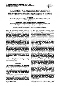
4. Experimental results 4.1 Data set construction In order to simplify illustration, we use data records having only three attributes, two numeric values and one categorical value. These records were generated as follows. We first created a set of 2D points, which contains 300 points and has three normal distributions as shown in Figure 1 (a). We then expanded these points to 3D by adding a categorical value to each point (see Figures 1 (b)). For this data set we deliberately assigned to the majority points in each part an identical categorical value and to the rest other categorical values. For instance the majority of points in the left low part in Figure 1 (b) are assigned categorical value C and


the rest in this part are assigned A or B. All assignments were randomly done.

(a) Three normal distributed pints in 2D. (b) Adding the categorical attribute to the points. Figure 1. The synthetic test data set with mixed numeric and categorical values

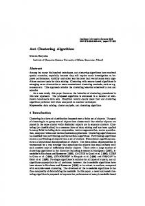
Note that the categorical value of a point does not indicate its class membership. In fact, these points have no classification at all. The categorical values simply represent objects in a third dimension, which is not continuous and has no order. 4.2 Simulations Figure 2 shows the clustering result of the proposed algorithm. It can be found that if a point has a categorical value A but is close the majority of points having categorical value B and far away from the majority points having categorical value A, the point is clustered together with the points, which have categorical value B in majority. In this case, the two numeric values determine the cluster of the point rather than its categorical value. However, if a point having categorical value A and surrounded by points having categorical value B is still not far away from the points with categorical value A, it is clustered with the points with categorical value A. In this case, its cluster membership is determined by its categorical value rather than its spatial location. Therefore, numeric and categorical attributes play an equivalent role in determining cluster memberships of the points.

Figure 2. The clustering result of our algorithm Figure 3. The convergence plots of our algorithm The online and offline performance of our GA-based clustering algorithm are plotted in Figure 3. The online and offline performance are defined as

∑

∑

1 t  1 N (i )  f ( g k ) t i =1  N k =1  1 t Poffline (t ) = max kN=1 f ( i ) ( g k ) t i =1 Ponline (t ) =

∑[

]

(16) (17)

where, t denotes the evolutionary generation. It is clear that our algorithm is converged quickly with the increasing of evolutionary generation, which shows good convergence performance.


4.3 Clustering a Large Data Set The purpose of this experiment was to test the scalability and validity of the algorithms when clustering large data sets. Large data sets were used in this experiment, which contains 80000 records, each record had 9 numeric and 11 categorical attributes.

(a) The CPU time versus number of clusters (b) The CPU time versus number of records Figure 4. The scalability and validity test experimental results of our algorithm

We tested two types of scalability of the algorithms on this large data set. The first one is the scalability against the number of clusters for a given number of objects and the second is the scalability against the number of objects for a given number of clusters. The experiment was performed on a PC with P4 1.7G CPU and 256M RAM. Figures 4 (a) shows the results of using our algorithm to cluster 80000 objects into different numbers of clusters. Figures 4 (b) shows the results of using this algorithm to cluster different numbers of objects into 50 clusters. The plots represent the average time performance of five independent runs. One important observation from these figures was that the run time of this algorithm tends to increase linearly as both the number of clusters and the number of records is increased.

5. Conclusions We have presented the genetic algorithm to cluster large data sets. The clustering performance of the algorithm has been evaluated using a large data set. The satisfactory results have demonstrated the effectiveness of the algorithms in discovering structures in data. The scalability tests have shown that the algorithm is efficient when clustering large complex data sets in terms of both the number of records and the number of clusters. These properties are very important to data mining. The emphasis of this paper is put on the issue that employs the genetic algorithm to solve the clustering problem. However, in using this algorithm to solve practical data mining problems, we still face the common problem: How many clusters are in the data? This will be a challenging topic for further research.

References [1] M. R. Anderberg. Cluster Analysis for Applications. Academic Press, New York, 1973. [2] B. Everitt. Cluster Analysis. Heinemann Educational Books Ltd., 1974. [3] Zhexue Huang, Michael K.Ng. A fuzzy k-modes algorithm for clustering categorical data. IEEE Trans. on Fuzzy Systems, 7(4): 446-452, August, 1999. [4] Zhexue Huang. A fast clustering algorithm to cluster very large categorical data sets in data Mining. Proceedings of the SIGMOD Workshop on Research Issues on Data Mining and Knowledge Discovery, Dept. of Computer Science, The University of British Columbia, Canada, pp.1-8. [5] R. Krovi. Genetic Algorithm for Clustering: A Preliminary Investigation. IEEE press, pp.504-544. [6] J. H. Holland. Adoption in Natural and Artificial System. Ann Arbor, MI: Univ. Mich. Press, 1975.
