[5], Koala [6], or Robocop [ref]) describe components as a set of interrelated models. Such models describe particular aspects of the components, such as the.
A Framework for Interactive Visualization of Component-Based Software Alexandru Telea, Lucian Voinea Department of Mathematics and Computer Science, Eindhoven University of Technology, Den Dolech 2, 5600 MB, The Netherlands {a.telea|l.voinea}@tue.nl Abstract In this paper, we advocate the use of visual tooling for the development and maintenance of component-based software systems. Our contribution is twofold. First, we demonstrate how an interactive visualization tool effectively supports understanding large component based software. Secondly, we show how to design such a tool in order to make it applicable for a wide range of component systems and investigation goals. We demonstrate our approach by several visualization scenarios for real-world systems.
1. Introduction Component based software systems have recently emerged as an alternative to traditional software system construction methodologies. Component systems attempt to accelerate software development and, in the same time, diminish production costs by assembling systems from existing software components. In this way, complex applications can be quickly built by maximizing the reuse of existing functionality, which is provided in the form of components. However promising, component based development can be a complex task. First, the design, development, and maintenance of reusable software components may be considerably complicated by the composability requirement, i.e. the ability of components to operate properly and effectively in a given composition context. Secondly, constructing applications from predefined components such that the resulting applications obey a number of functional and/or non-functional requirements can be a challenging task. Most component architectures (e.g. COM [4], CORBA [5], Koala [6], or Robocop [ref]) describe components as a set of interrelated models. Such models describe particular aspects of the components, such as the
execution, functionality, documentation, behaviour, and resource consumption. As component-based applications become increasingly complex, the question of how to effectively understand both their structure and behaviour becomes harder to answer. Typical questions that frequently arise when developing component-based systems are: How do component models or their instances (i.e. the applications) evolve in time? How can one check that a given component instance matches a given component model (or set of models)? How cleanly designed (e.g. modular) is a given system? How can one find out specific design problems in a given component instance and/or model? Such questions can be partially answered by applying several metrics on the systems at hand, such as computing the coupling, fan-in, or fanout of a system of interconnected components to assert the system’s modularity [3]. However, in most cases one does not know beforehand which metrics to compute. Understanding the computed metrics can be hard even for a moderately sized system of a few tens of components and becomes a challenge for systems of hundreds of components or more. Finally, many objectives, such as understanding a system’s evolution in time, are not easily quantifiable in metrics, but require a different type of insight. We address the above questions by advocating an interactive visualization approach using customizable tooling. We propose a software framework for interactive visualization and exploration of the structure, properties, and behaviour of componentbased. Our framework implements several visual metaphors, or tools, that can be used to understand component-based architectures to up to hundreds of components. Users can freely specify both the component data to be examined (i.e. what they want to visualize) and the visualization scenarios (i.e. how they want to view the data). We achieve this high customizability by using a component architecture for our framework. We demonstrate our solution by
visualization scenarios using real-world component architectures. The remainder of this paper is as follows. In Sec. 2 we describe how we model a problem, i.e. understanding a component-based system, in our framework. Section 3 details the design of our framework, showing how it effectively and efficiently supports the requirements stated in Sec. 2. Section 4 demonstrates the use of our framework on several real-world component systems. Finally, Section 5 concludes the paper.
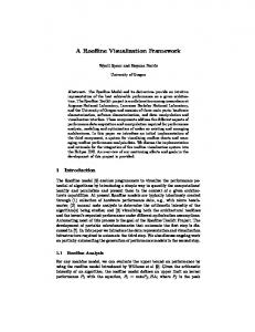
2. Problem Modeling To be successful, our visualization framework should: • Work on software systems based on different (ideally, any) component architectures (R1) • Support a wide range (ideally, any) type of queries such as the ones sketched in Section 1 (R2) Problem Model Component Model
Scenario Model
attribute 1 attribute 2 attribute 3 attribute n
operation 1 operation 2 operation 3 operation n
Figure 1: Problem model We model a problem in our visualization framework by two elements: a component model (CM) and a scenario model (SM) (see Fig. 1). Concerning the first requirement (R1), one of the main respects in which software architectures differ from each other is their component model. So far, there is no ‘mainstream’ component model that easily integrates other models. Moreover, component models evolve and/or are open to extension. For the needs of our visualization framework, we use a very simple, yet generic component model: A component is a set of named textual attributes. Every attribute describes some property, such as the component’s number of lines of code, required memory consumption, executable platform, version number, or component interdependencies, such as “provides”, “requires”, or “contains” relations. Obviously, existing CMs easily map into our description. For example, the executable model of a component in the Robocop architecture consists of several services that provide several interfaces, or ports ([xxx]). A similar port concept exists in the COM and CORBA component models too
[4,5]. In our simple CM, these ports would translate to a set of named attributes. To keep our model simple, we don’t strongly type our attributes in any way. Whereas the component model describes what we wish to visualize, the scenario model (SM) describes how we want to construct the visualization. Specifically, the SM consists of a set of operations. Each operation describes an action that is part of the visualization. For example, a typical visualization scenario consists of the following operation sequence: • read some component software description; • select a subset of interest from the whole dataset; • compute some metrics on the selected subset; • represent visually the selected subset, with the computed metrics; • specify how the visualization reacts to the user interaction. Users with different concerns (questions) and/or different component systems will require different visualization scenarios consisting of different operations. For example, the metric operations used for Java-based component software may be different than the ones used for one based on C or C++. In this sense, the syntax and semantics of the operations in the scenario model correspond to the syntax and semantics of the CM respectively. To be effective, our visualization framework must support several scenario models implementing a wide range of operations (R2). In the next section we describe the classes of operations our framework supports and explain the design choices we took to ensure the requirements (R1) and (R2).
3. Visualization Framework Architecture The architecture of our visualization framework consists of two main elements: a data model (DM) and an operation model (OM). The operations (part of SMs, described in Sec. 2) communicate with each other via the shared data model (Fig. 2). The data model holds component instances of the CM described in Sec. 2. The DM is implemented in C++ for efficiency reasons. The OM is implemented partly in C++, for efficiency, and partly in the interpreted Tcl language for flexibility. We next describe both the DM and OM.
3.1. Data Model Data to be visualized consists of three elements: structure, attribute values, and selections, as follows.
Structure and attribute values refer to the instantiation of the relational, respective non-relational attributes in the CM. We can see the structure as a graph whose nodes are the component instances and arcs the relations between these instances (Fig. 2). This graph can have any topology, as there are no constraints on the relations between components. The attribute values represent concrete instances of the CM attributes. They may take values of several basic types (int, float, string, pointer, and arrays thereof). If desired, specific problem models may place topological and/or value constraints on the structure and attribute values respectively and check them via operations in their SM (see Sec. 3.2).
Figure 2: Framework architecture Selections, defined as named sets of nodes and edges (i.e. component and relation instances respectively), are the last element of our framework’s data model. Selections allow specifying the data elements on which visualization operations are executed. To make our framework flexible, we decouple the selection specification (which are the data to operate on) from the operations' definitions (what to do with the selected data). All operations in our framework communicate with each other only via selections. Practically, selections play the role of (named) input and output variables in dataflow programming. Let us give an example: Given some component-based software, we want to visualize all component instances thereof, which are of a given type Package. This visualization scenario can be expressed as the following sequence of three operations: 1) Inp = readData(input) 2) Out = selectOnValue(Inp,type,Package)
3) display(Out)
The first operation readData reads all component data from some input file input and places it in the selection Inp. The second operation produces the selection Out containing all data elements in Out whose attribute called type has the value Package, i.e. all component instances of package type. Finally, the third operation display produces a visual image of the selected subset Out.
3.2. Operation Model Operations, already introduced in the previous section, are of three classes (see also Fig. 2): • Editing: change the structure and/or attribute data • Selection: change the selection set • Mapping: map selections to visual objects In the previous example (Sec 3.1), readData is an editing operation, as it creates new nodes and edges in the data model, when reading the input data; selectOnValue is a selection operation, as it creates a new selection; and display is a mapping operation as it maps the selection Sel to visual objects. Operations may have three types of parameters: • Selections: specify the selections to be read/written • Attributes: specify the attribute names from the CM to be read/written • Values: specify other operation-specific parameters, such as thresholds, flags, options, etc. This above operation model has several advantages. As operations are explicit about which data elements they change, the framework can perform automatic updates. For example, if some selection Sel changes, all data viewers (discussed in Sec. 3.2.3) that monitor Sel are automatically updated. The fixed operation interface (selections, attributes, values) allows the framework to automatically construct graphics user interfaces (GUIs) for all operations, in which users can set operation parameters and monitor results. Overall, this allows users to easily program new operations and incorporate them with minimal effort in SMs of the framework, as detailed in Sec. 3.3. We next discuss the three operation types, give examples for each type, and show how the genericity and flexibility requirements set to our framework are met. 3.2.1. Selection Operations
Selection operations are the main instrument used to navigate through large component architectures. Given one or several input selections, a selection operation produces an output selection containing component instances and relations (i.e. nodes and edges) that match the desired criteria. Several examples follow. Conditional selections gather all elements in the input whose attribute values match some condition. In this way, filters such as “get all component instances of a type T” or “get all component instances providing an interface I” can be readily implemented. Call graph selections gather all component instances reachable from a given component via a given function or service call. Level selections (called 'horizontal slices' in the reverse engineering literature [Wong, 1999]) are useful to visualize multi-layer software architectures at a given level of detail, by gathering all component instances in a given architectural layer. Tree selections (called 'vertical slices' in [Wong, 1999]) gather all component instances and containment relations reachable from an input selection, and are useful for visualizing subsystem structures or change propagation [Marshall et al., 2001]. Finally, boolean selections allow combining existing selections via intersection, union, etc, and allow creating arbitrarily complex filters from simple building bricks. 3.2.2. Editing Operations Structure editing operations construct and modify the graph. Such operations include reading several data file formats such as RSF [8], DOT [9], and GXL [2]. Visualizing some custom component-based software amounts thus to program a new operation for reading the desired data format. If the data at hand is too large to be directly visualized (e.g. there are too many components), aggregation operations can be used to simplify it. These take the data (nodes and edges) in an input selection and replace them with a unique ‘cluster’ node. The input selection can be programmatically constructed, e.g. by automatic clustering methods, or can be the output of user interaction, described in Sec. 3.2.3. Attribute editing operations modify the attribute values of component instances but not the relations, i.e. the graph structure. Such operations are architectural metrics, e.g. component coupling strength, number of provisions, requirements, and internalizations [8]. Metrics can compute new attribute values for each component instance, such as the above examples, or single values for whole selections, such as global subsystem quality metrics. Decoupling the selection of the metric’s input from the metric
computation itself allows applying any metric on any subset of components (selection), which is not the case in other software visualization tools [8, 11]. Moreover, explicitly specifying the attribute names that store the metric allows easy run-time prototyping of various metric combinations. For example, one can compute several metrics, store them in several attribute values, and then interactively cycle through the computed metrics to e.g. visually compare them. Layout operations (or layouts briefly) are the first step in bringing the abstract component data to a visual representation. Given that component instances and their relations form a graph (as explained in Sec. 3.1), a very natural way to visualize these is to draw this graph. Drawing the graph involves two steps: assigning a geometric position to every node and edge; and choosing a graphic symbol to draw every node and edge. The first step, called laying out the graph, is performed by layout operations. In detail, layouts compute geometric position attributes for the nodes and edges in a given input selection. The second step, called mapping the graph, is discussed separately in Sec. 3.2.3. Decoupling the drawing in the layout and mapping steps has several benefits. First, we can layout different subgraphs corresponding to different component subsystems separately. For example, containment relations between component instances (vertical slices, Sec. 3.2.1) are best visualized using a tree layout (Figure 6 top). Call graphs or horizontal slices (Sec. 3.2.1) are best visualized using a so-called spring embedder layout [9]. Second, we can precompute several layouts e.g. to quickly switch between them. This is useful for large graphs (thousands of component instances) whose layouts may take up to minutes. Finally, we can cascade different layouts on the same position attributes, e.g. to interactively refine an existing layout. An example of cascading is the nested layout described next. Nested layouts are useful to visualize both containment and association (“provides”, “requires”) relations of a component architecture. If we draw components as boxes, we depict containment (“A contains B”) by drawing B’s box inside A’s, and association (“A provides/requires B”) by drawing a line between A and B (see Figure 5 and Figure 6). To produce such results, we lay out separately the sub-components of every component instance using the spring embedder layout and then lay out recursively the bounding boxes of the containing nodes. Nested layouts produce images similar to package UML diagrams and have proven to be very helpful in many applications [9,10], as they are quite
familiar to software engineers. Users can easily combine simple layouts as the building bricks for the more complex layouts. Adding new layouts to our framework is reasonably simple. The implementations of the spring embedder and tree layouts we use in our framework [9] exceed 50000 C lines. Adding them in a black-box fashion required less than 100 C++ lines for each. Our custom layouts, such as the nested layout, have each fewer than 200 C++ lines. 3.2.3. Mapping Operations So far, we described how to read data (Sec. 3.2.2), select subsets of interest (Sec. 3.2.1), and assign geometric positions for drawing it (Sec. 3.2.2). Mapping operations, discussed here, allow users to customize the way data is finally drawn to produce the visualization, and how users can interact with the visual objects. Creating visual representations of our data model must obey two requirements. First, users must be able to easily customize the way objects are drawn. Second, the framework must cope with drawing and interacting with potentially complex drawings of thousands of visual objects in real time. To fulfill these requirements, we designed an architecture consisting of four elements: mappers, viewers, glyph factories, and user actions (Fig. 3). The implementation is based on the C++ toolkit Open Inventor that provides advanced mechanisms for rendering and interacting with large 3D models [7]. The mapper is the central element of the mapping subsystem. It is responsible for creating 2D or 3D visual representations of the data model. We have implemented several mappers, as follows. The glyph mapper creates an iconic symbol, also called a glyph, for each component instance (node) and relation (edge) in its input selection, and places these glyphs at the
geometric coordinates provided by attribute values previously computed by a layout operation (Sec. 3.2.2). The glyph mapper allows customizing the drawing of every individual node or edge glyph, as follows. For every node and edge it maps, the glyph mapper calls a glyph factory software component, which builds the desired glyph visual representation and returns it to the mapper. The glyph factory sets the glyph's graphical properties (color, shape, size, annotation, transparency, and so on) from the attributes of the mapped node or edge. Users can thus customize the appearance of every single node and edge in the visualization by simply switching between various predefined glyph factories. Most such factories are programmed in the scripting language Tcl, so users can even edit them on the fly, to obtain complete customization. The usage of glyphs is exemplified by applications in Sec. 4.1 (Figure 5) and 4.2 (Figure 6). A second type of mapper is the splat mapper. Instead of drawing nodes and edges explicitly, as the glyph mapper does, the splat mapper produces a height map, or 3D plot. The height map shows the density of nodes per unit area, following the placement produced by e.g. a spring embedder layout. Splat mappers effectively visualize large tightly connected graphs, such as the ones arising from the “provides” or “requires” relations in component architectures. Drawing all nodes and edges of such graphs separately often produces cluttered images when high coupling is present, i.e. there are too many relations in the system. Instead, a height map is effective for spotting tightly coupled subsystems, as component instances in these subsystems are ‘gathered’ together by the spring embedder layout. The splat mapper is demonstrated by applications in Sec. 4.3 (Figure 7).
Figure 3: Mapping and visualization subsystem The third component of the mapping subsystem is the viewer. Viewers (Figure 5) display the output of mappers and also allow mouse-based 2D and 3D
navigation (zoom, pan, rotate, fly through) in the displayed data, as well as interaction with the displayed data. Viewers can be thought as operations
(Sec. 3.2) having an input and an output selection and an attribute argument. The data in the input selection is displayed using a mapper. When the user selects the displayed objects, using the mouse, the viewer adds the selected objects in its output selection. The output selection can be then passed as input to any of the framework’s operations (filtering, editing, viewing, etc). In this way, users can easily both navigate the complete data to get an overview and select some subsystem of interest to examine it in more detail. Finally, viewers allow specifying a so-called user
3.3. Component Architecture For our framework to be effective in practice, users must avail of a wide range of problem models, consisting of component models (CMs) and scenario models (SMs). Writing a CM for a given componentbased system is usually easy, as it involves translating the native application CM to our simple CM format (Sec. 2). Writing a custom SM involves crafting appropriate editing, filtering, and mapping operations that support the questions specific to the system being analyzed. In order to simplify the usage of such operations (i.e. writing, packaging, browsing, and customizing them), we introduced a simple component-based metaphor in our framework. All customizable software elements in our framework (operations, viewers, glyph factories, and user actions) are implemented as components with fixed interfaces. Components are declared in Tcl and may be implemented either in Tcl or compiled C or C++. To exemplify, we sketch next the declaration of the operation component selectOnValue introduced in Sec. 3.1:
action. This is an operation that is executed every time the user performs mouse-based selection in a viewer, and receives as input the viewer’s output selection. By customizing the user action, a wide range of exploration scenarios can be implemented. For example, a user action can pop up a second viewer displaying the data the user selected in a first viewer, as demonstrated by the application in Sec. 4.2.
whose value should equal value. The info declarator gives some information text to be displayed in the component’s GUI. Finally, the exec declarator is the name of a Tcl procedure that implements the operation’s functionality. Given this declaration, the visualization framework automatically constructs a component GUI and adds the component in a visual browser. Figure 4 (upper half) shows the browser in which we selected the selectOnValue component, whose GUI is shown in the lower half of Figure 4.
component selectOnValue { type operation library filters selections { input output } attributes { name value } info “Selects by attribute value” proc exec { input output name value } { … implementation … } }
The first declarator type gives the component’s type, i.e. operation in this case. The library declarator specifies the component library this component is part of. Components can be organized in hierarchical component libraries, much as class libraries in OO languages. The selections declarator gives the operation’s selection arguments, in this case the output. The selections input and attributes declarator gives the operation’s attribute arguments, in this case the attribute name
Figure 4: Component browser and GUI Creating SMs is easily done by packaging those components that should be used together for a given problem domain. A typical visualization proceeds then as follows. The user loads the desired PM, e.g. “Architectural metrics for Java-based software”, from an existing set of pre-packaged PMs. Next, the concrete data to be visualized is loaded, in this case an architectural description of some Java-based system. Next, the user browses through the components made
available by the loaded PM, selects the desired ones, and applies them on the loaded data in the desired order, to gain the desired insight. No programming experience is needed here, as all actions are done just via the component GUIs.
longest/shortest metric bars. Displaying the four metrics along each other with the bar chart glyph allows easy comparison of the metrics for the same component. Using the same color for the same metric allows comparison of that metric between different components.
4. Applications In this section, we demonstrate the use of our visualization framework with three real-world applications using component-based software.
4.1. Architectural Metrics In this application, we visualize several architectural metrics computed by the software analysis tool SAAT [3] on a given software system (Figure 5). Our system representation consists of a logical view, containing structural inter-component relations, and a scenario view, containing use cases describing specific system tasks. We use a nested layout (Sec. 3.2.3) to represent the use cases, scenarios, and components: If component C is in scenario S, its visual representation is contained in C’s visual representation. For use cases and scenarios, we use simple box glyphs. For the system we study, containment has just three levels (components in scenarios, scenarios in use cases). However, our nested layout can accommodate in principle any number of containment levels. Intercomponent relations (method calls) are drawn as lines. If the same element (e.g. component) appears in several scenarios, it is separately drawn in every scenario box. This matches the representation expected by system architects. When the user selects a component in a scenario with the mouse, all visual representations of that component in all scenarios it occurs are automatically highlighted (Figure 5). This is easily implemented by a custom user action (Sec. 3.2.3). This allows easy comparison of the behavior of a given component in different scenarios. For components, we use a special glyph that shows four metrics: coupling, inverse coupling, fan in, and fan out. These are displayed as a four (individually colored) bar chart in 3D. Finding outliers, i.e. components with high/low metrics, is easy, as these have the
Figure 5: Architectural metrics
4.2. Multiple Views in Reverse Engineering We visualize now a component-based mobile phone architecture from Nokia [ref vissym]. The data comes from reverse engineering an existing software system of several hundred components. First, we use a filter to select all component instances and their containment relations. We display these using a tree layout and a glyph colored by the component type (Figure 6 top). When the user selects, with the mouse, some components in this viewer, we display them and all contained sub-components in a second viewer using a nested layout (Figure 6 bottom). This shows us both containment relations (boxes in boxes) and call relations (lines between boxes). We easily implement the above by a user action for the first viewer (Sec. 3.2.3).
Figure 6: Subsystem containment (top) and dependencies (bottom) This scenario, constructed in just a few minutes, allows us to see which are the 'interface' components through which Subsystems 1 and 2 communicate. We also see that lower level components (innermost boxes in the nested layout) do not make cross-system calls, a desired property of software architectures.
4.3. Visualizing Provisions In this application, we visualize the provision, or “is called by”, relations in a Java-based software system of about 2000 components. Since the provision relations graph is dense, visualizing it using a spring embedder layout and glyphs (e.g. boxes and lines) produces a cluttered image. Instead, we use a splat mapper (Sec. 3.2.3). The dots in Figure 7(left) show the components’ positions computed by a spring embedder. The shaded image shows the density field computed as number of packages times number of provision relations per unit area. Figure 7(right) shows the same field as a height plot. We can see two ‘hot spots’ in the left image, corresponding to the two peaks in the right image. These correspond to the most called classes in the system, i.e. String and ListIter. Other hot spots correspond to other frequently used components. A similar scenario can be built to visualize component requirements.
Figure 7: Visualizing provisions
5. Conclusions The aim of this paper is to demonstrate the usefulness of visual tooling for the development and maintenance of component-based software. Our contribution is twofold. First, we demonstrate the usage of our visualization tool in three scenarios for real-world software systems. Secondly, we show how we used a component based tool architecture to make the customizability of our tool simple for end users. This lets us define a visualization scenario in minutes by assembling pre-packaged components such as data editing, filtering, rendering, and user actions. Having this stable framework, our main focus now is to
construct more visualization components and apply them to support both forward and reverse engineering of large component-based software systems.
6. References [1] The Robocop paper please !!!
[4] Box, D, Essential COM, Object Technology Series, Addison-Wesley, 1997 [5] Mowbrai, T. and Zahavi, R, Essential Corba, John wiley & Sons, 1995 [6] Van Ommering, R., F. van der Linden, J. Kramer, and J. Magee, “The Koala Component Model for Consumer Electronics Software”, IEEE Computer, 33 (3), IEEE CS Press, 2002, pp. 78-85. [7] Wernecke, J. The Inventor Mentor: Programming Object-Oriented 3D Graphics, Addison-Wesley, 1993. [8] Wong, K., S. Tilley, H. Muller, and M. Storey, “Structural Redocumentation: A Case Study”, IEEE Software, 12 (1), 1995, IEEE CS Press, pp. 46-50. See also Rigi User’s Manual, Dept. of Computer Science, Univ. of Victoria, Canada. [9] North, S. C. and E. Koutsofios, “DOT and NEATO’s User Guide”, AT&T Bell Labs Reports, http://www.research.att.com, 2000 [10] Riva, C., A. Maccari, A. Telea, “An Open Visualisation Toolkit for Reverse Architecting”, Proc. IWPC, IEEE CS Press, 2002 [11] Kazman, R. and Carriere, J., “Rapid Prototyping of Information Visualization using VANISH”, Proc. IEEE InfoVis, IEEE CS Press, 1996, pp. 91-98
[2] Marshall, M. S., Herman, I., and Melançon, G., “An object-oriented design for graph visualization”, Software: Practice and Experience, 31(8), John Wiley & Sons, 2001, pp. 739-756. [3] Muskens, J., SAAT: Software Architectural Analysis Tool, Master’s Thesis, Department of Mathematics and Computer Science, Eindhoven University of Technology, 2002