to access data via high-level query languages, and it is the responsibility of ...... Rule 3b: Let Gbe a graph, ek;l a node, and Cost(SQ1k;l)+Cost(ek;l) Cost(SQ1).
Nationaal Lucht- en Ruimtevaartlaboratorium National Aerospace Laborator y NLR
NLR TP 97563
A framework for multi-query optimization Sunil Choenni and Martin Kersten
DOCUMENT CONTROL SHEET ORIGINATOR'S REF. TP 97563 U
SECURITY CLASS. Unclassified
ORIGINATOR National Aerospace Laboratory NLR, Amsterdam, The Netherlands
TITLE A framework for multi-query optimization
PUBLISHED IN Proc. COMAD '97 8th Int. Conference on Management of Data published by Springer, 1997
AUTHORS Sunil Choenni and Martin Kersten
DESCRIPTORS Architecture (computers) Algorithms Computerized simulation Data base management systems Data bases
DATE October, 97
pp 30
ref 19
Data processing Information retrieval Information systems Optimization Query languages
ABSTRACT In some key database applications, a sequence of interdependent queries may be posed simultaneously to the DBMS. The optimization of such sequences is called multi-query optimization, and it attempts to exploit these dependencies in the derivation of a query evaluation plan (qep). Although it has been observed and demonstrated by several researchers that exploitation of dependencies speed up the query processing, limited research has been reported how to benefit from multi-query optimization, taking the capabilities of existing query optimizers into account. This is exactly the topic of this paper. Since existing optimizers are able to optimize queries in which a restricted number of basic operations appears, e.g., number of joins is limited to ten, and the optimization of a query is relatively expensive, we attempt to profit from multi query optimization under the condition that queries are passed only once and separately to the optimizer. We propose a two-step optimization procedure. In the first step, we determine, on the basis of the dependencies between queries, in which order they should be specified and what results should be stored. In the second step, each query is passed separately to an optimizer.
217-02
-3NLR-TP-97563
Summary In some key database applications, a sequence of interdependent queries may be posed simultaneously to the DBMS. The optimization of such sequences is called multi-query optimization, and it attempts to exploit these dependencies in the derivation of a query evaluation plan (qep). Although it has been observed and demonstrated by several researchers that exploitation of dependencies speed up the query processing, limited research has been reported how to benefit from multi-query optimization, taking the capabilities of existing query optimizers into account. This is exactly the topic of this paper. Since existing optimizers are able to optimize queries in which a restricted number of basic operations appears, e.g., number of joins is limited to ten, and the optimization of a query is relatively expensive, we attempt to profit from multi query optimization under the condition that queries are passed only once and separately to the optimizer. We propose a two-step optimization procedure. In the first step, we determine, on the basis of the dependencies between queries, in which order they should be specified and what results should be stored. In the second step, each query is passed separately to an optimizer. Keywords: data management, multi-query optimization, architectures, exploiting interdependencies between queries.
-4NLR-TP-97563
Contents 1
Introduction
5
2
Architectures for multi-query optimization
8
3
Query processing
11
3.1
Preliminaries & assumptions
11
3.2
Model
11
4
Exploiting interdependencies between queries
15
4.1
Common subquery
15
4.2
Approach
16
4.2.1
Phase 1
17
4.2.2
Phase 2
18
5
An algorithm
21
6
A case study
23
7
Conclusions & further research
28
10 Figures
(30 pages in total)
-5NLR-TP-97563
1 Introduction Query optimization has been recognized as an important area in the field of database technology [Ref 18], especially since the introduction of relational systems. Relational systems offer the user to access data via high-level query languages, and it is the responsibility of the system to select efficient plans to process queries, called query evaluation plans (qeps). A qep describes in which order basic operations, such as selections, projections, joins, etc., should be evaluated to obtain the query answer. Much research has been devoted to select automatically efficient qeps [Ref 7]. Since the first and most important database applications were produced in administrative areas, research on query optimization was primarily focussed to meet their performance requirements. An assumption often implicitly made is that these applications give mainly rise to independent queries with a limited number of basic operations. This makes it possible to select efficient qeps by a complete enumeration or by applying a few effective heuristics. For example, the number of joins involved is generally less than ten for those applications. As the variety of database applications grows rapidly, its impact on the performance requirements and the pattern of queries passed to the optimizer poses new research challenges. In database applications, such as data mining and decision support systems, a sequence of interdependent queries are passed simultaneously for processing [Ref 3]. Often, complex queries are split into a number of simpler queries whose results are used by the application to derive the desired result. The simpler queries are passed simultaneously to the DBMS for processing. Optimizing such interdependent queries separately leads to performance that is far from optimal. This has led to several approaches to exploit the dependencies between queries such as illustrated by [Refs 1, 8, 9, 10, 12, 13, 16]. In [Ref 8], the author describes how common subexpressions can be detected, and used according to their type (e.g., joins, selections, etc.,). In [Ref 10], necessary and sufficient conditions are discussed to compute query results from previously executed queries. In [Refs 12, 13], a framework is provided to derive a common query graph from individual query graphs belonging to individual views, in an attempt to speed up view processing. In the common query graph, different ways are presented to produce the result of a view. Then, the effect of indices on the common query graph is studied, and a set of indices is selected. In [Ref 9], a two-step optimization is proposed. In the first step, an analysis of database and query characteristics is performed, and a grouping of queries for simultaneous processing is determined. In the second step, each group of queries is processed in the order determined at the first step and intermediate results are stored on disk. In [Ref 16], two algorithms are described for multi-query processing. In the first algorithm, an optimal access
-6NLR-TP-97563
plan is generated for each query. Then, a global access plan is obtained by merging the optimal access plans of each query, taking common subexpressions into account. In the second algorithm, a number of access plans for each query is considered. Then, on the basis of heuristics an access plan is chosen for each query such that all common subexpressions found among the queries are used effectively. In [Ref 1], it has been demonstrated that rewriting a set of related expressions in the context of each other, such that no resulting common subexpression is weaker than any of the related expressions, is superior than rewriting techniques that induce common subexpressions that are weaker than the set of related expressions. In this paper, we address the following problem: how to restructure a sequence of queries such that it can efficiently be processed using the optimizing techniques available in the query optimizer of existing DBMSs. The idea of our approach is to determine an order in which a sequence of (sub)queries should be processed, such that we may profit from the dependencies between queries in processing them. Then, each query is passed separately to the optimizer, and the optimizer selects an efficient query evaluation plan. Although we consider a restricted class of conjuctive queries, i.e., queries whose WHERE clause consists of a conjunction of selections and equi-joins, this class contains the most common type of queries. Furthermore, this type of queries is also significant for complex queries, since complex queries are often split into a set of simple queries before processing [Ref 1]. Since disk accesses are still the main cost factor for the above-mentioned type of queries [Refs 2, 4, 14], disk accesses will be taken as processing unit. What distinguishes our approach to optimization of interdependent queries from the before-mentioned efforts is that we use an existing optimizer, and view to it as a ‘black-box’. This approach avoids re-development of a complex query optimizer and is adaptive to emerging techniques for query optimization. However, one should be aware of the following limitations of using an existing optimizer. First, as noted already, optimizers are able to handle queries efficiently with a limited number of basic operations only. Approaches based on the integration of queries into a single query graph, such as in [Refs 1, 8, 12, 13], are not suitable when using existing optimizers. Passing large query graphs would burden an optimizer with an infeasible task. Second, the optimization of a query is a time consuming task [Refs 2, 6]. Approaches based on many invocations of an optimizer for a single query, such as in [Ref 16], will considerably slow down the optimization process. The remainder of this paper is organized as follows. In Section 2, we discuss four possible architectures to integrate techniques that exploit dependencies between queries and conventional optimizers. In Section 3, we discuss a model how to reuse existing output of queries in processing
-7NLR-TP-97563
new queries. In Section 4, we elaborate our approach, and, in Section 5, we introduce an algorithm based on this approach. The effectiveness of our approach is shown by a realistic case study in Section 6. Finally, Section 7 concludes the paper.
-8NLR-TP-97563
2 Architectures for multi-query optimization In this section, we discuss a number of architectures to integrate techniques that exploit dependencies between queries and conventional optimizing techniques. For each architecture, we point out the strong points and flaws. In Figure 1, we have depicted four possible architectures. We note that variants of architectures 1(a) and 1(b) have been introduced in [Ref 16]. query multi-set of queries Conventional Optimizer Advanced Optimizer
qep Reuse Manager
global evaluation plan
qep’ (a) multi-set of queries
Reuse Manager
(b) multi-set of queries reuse information
Order Manager
Reuse Manager
order part of a qep Conventional Optimizer
qep (c)
qep
part of a qep
Conventional Optimizer
qep (d)
Fig. 1 Architectures
In Figure 1(a), a multi-set of queries arrives at the optimizer. The optimizer selects an efficient global evaluation plan, which contains the processing strategy for all queries. Then, the plan will be executed. In this architecture, conventional optimization techniques and optimization techniques based on dependencies between queries are strongly integrated. We note that the rule base or cost model used by optimizer will become more complex, since the effects that dependencies between queries will have on an evaluation plan should be modelled as well. Such an architecture is suitable for the development of an optimizer from scratch. In Figure 1(b), a conventional optimizer selects for each query an efficient qep. Then, all qeps are passed to a reuse module, which attempts to profit from the common parts (caused by the dependencies) by computing them only once and to reuse them in qeps. Consequently, query eval-
-9NLR-TP-97563
uation plans are rewritten before being executed. Query evaluation plans are based on the available storage structures and access structures in a database management system. A qep produced by a Ingres optimizer may differ from a plan produced by Oracle optimizer. Since the reuse manager attempts to optimize a number of plans by reusing the results of common parts, it is not interested in all details provided by a specific optimizer, such as how a relation is accessed. So, it abstracts from the details and focus on the information relevant for the reuse of earlier computed results, as illustrated in [Ref 16]. Once the re-use parts are determined, the abstracted evaluation plan should be augmented with the processing details, in order to be executed by the database system. In fact, architecture 1(b) requires another interface between the optimizer and reuse manager for each kind of database system. Another disadvantage of this architecture is that an optimal plan generated by the conventional optimizer for a query may be killed by the re-use manager, making the effort of the conventional optimizer wasteful. This may happen, e.g., when the output of a query is solely derived from earlier computed results. In this case, a plan generated by an optimizer becomes useless. In Figure 1(c), a multi-set of queries arrives at the reuse manager. The reuse manager determines in which order the queries are to be passed to the conventional optimizer and how to reuse earlier computed results. In fact, the reuse manager determines a part of the qep. An advantage of this architecture above architecture 1(b) is that in principle the same reuse manager can be used for each kind of database system. Furthermore, since the reuse manager determines a part of the qep, it relieves the task of a conventional optimizer. In Figure 1(d), the order manager receives a multi-set of queries and chooses an order of execution. Then, it passes the queries to a reuse module to determine the best way to reuse earlier computed results given this order. After receiving the requested information, it passes each query with the information on how to reuse earlier computed results to the optimizer. The optimizer passes on its turn a query evaluation plan to the order module. On the basis of the evaluation plans, the order module may choose another order and the whole procedure may be repeated. This architecture is comparable with architecture 1(c). The difference with architecture 1(c) is that the task of determining an order in which queries should be executed and what and how to reuse earlier computed results are made explicitly in this architecture. In the remainder of this paper, we will elaborate and implement architecture 1(c) for the following reasons. Commercial database management systems can efficiently handle queries in which a limited number of basic operations appears, e.g., no more than 10 joins [Ref 17]. For example, the optimization algorithm used in System R [Ref 15] becomes infeasible if the number of joins
- 10 NLR-TP-97563
is larger than 10 [Ref 17]. Since we attempt to use existing optimizers in the optimization of interdependent queries, we avoid large query graphs. Therefore, we reject architecture 1(a). Since query optimization is a time consuming process, we attempt to limit the number of invocations of an optimizer. Consequently, architecture 1(d) is rejected as well. Finally, we choose architecture 1(c) above 1(b) for the reasons discussed above, namely, the same reuse manager can be used for each kind of database system and it relieves the task of a conventional optimizer.
- 11 NLR-TP-97563
3 Query processing This section is devoted to a model to store output of queries and how to use them in query processing. Before presenting this model, we briefly outline some preliminaries in Section 3.1. 3.1 Preliminaries & assumptions
R is defined over some attributes, such as, �1 ; �2 ; :::; �n , and is a subset of the Cartesian product dom(�1 ) � dom(�2 ) � ::: � dom(�n ), in which dom(�j ) is the set of values assumed by �j . A restricted class of conjunctive queries, We deal with relational databases. Each relation
i.e., a conjunction of selections and equi-joins in a WHERE clause, is considered. A selection
R:�i op constant, in which op 2 f=; 6=; ; �g. An equi-join is a predicate of the form R1 :�i = R2 :�j . We do not consider projections to simplify our analis a predicate of the form
ysis without invalidation of the obtained results. Incorporation of projections into our approach is straightforward. Observe that a disjunction of predicates in a WHERE clause of a query can be replaced by a number of queries, for which the WHERE clause consists of a conjunction of predicates. Although we restrict ourselves to a special class of queries, this class contains the most common types of queries. This class of queries is also significant for complex queries, since a complex query is often split into a number of queries of the above-mentioned types [Ref 1]. Furthermore, we assume that a database resides on disk. For the above-mentioned class of queries, the processing cost depends on the number of disk accesses and CPU costs. However, the dominant cost factor is still disk accesses [Refs 2, 4]. Therefore, we take disk accesses as cost unit. Finally, we assume that a relation is stored as a heap, and no indices are allocated to attributes. We note that a data warehouse, which generally maintains historical information, is a typical application that is implemented in this way. 3.2 Model Our approach for multi-query optimization exploits the dependencies between the queries in a sequence. To speed-up query processing, (intermediate) results of queries are temporarily stored and reused. Although our approach can be targeted to different models that store intermediate results, we describe a model to store and reuse intermediate results for illustrative purposes. We assume that each tuple in a relation has a unique tuple identifier (tid). Instead of storing tuples that qualify as intermediate results, we store its tid in main memory. For reasons of simplicity, we assume that a main memory is large enough to store all tids that qualify as intermediate results1 . 1
If this assumption appears to be false, several strategies can be used to control the main memory by discarding
results. One strategy might be to discard the results that will be not used in future.
- 12 NLR-TP-97563
So, an intermediate result can be regarded as a relation
T , called tid-relation, in which attribute
�i assumes tid values of relation Ri . For example, storage of intermediate results due to a join between two relations Ri and Rj leads to the storage of a tid-relation Ti;j having two attributes �i and �j , in which �i and �j assume tid values of Ri and Rj respectively. A consequence of this storage model for intermediate results is that whenever one needs a tuple, this should be retrieved from disk. Before illustrating how to use tid-relations in query processing, we present a definition for the intersection of two tid-relations that resides in main memory. Definition 3.1: Let TR1 ;R2 ;R3 :::;Rn
�1 ; �2 ; �3 ; :::; �n ) and TS1 ;S2 ;S3;:::;Sm = ( 1 ; 2 ; 3 ; :::; m ) be relations, in which dom(�i ), i � n, and dom( j ), j � m, are the set of tid values that appears in relation Ri and Sj , respectively. Let u:� represents the value of an attribute � in a tuple u. Then, the intersection of TR1 ;R2 ;R3 :::;Rn and TS1 ;S2 ;S3 ;:::;Sm is =(
\(TR1 ;R2;R3 :::;Rn ; TS1 ;S2;S3;:::;Sm )
=
fuvju 2 TR1 ;R2;R3 :::;Rn ; v 2 TS1;S2;S3;:::;Sm ; 8�i; j : dom(�i ) = dom( j ) ) u:�i = v: j g 2
We note that the intersection of two tid relations results into a relation in which attributes that are defined on the same domain have the same value. Consider the two relations R and S below. Assuming that �2 and 1 , and �3 and 2 are defined on the same domain, the result of the inter-
section is a relation with one tuple as given below. R:
α1
α2
100
200 301
α
S:
3
β1
β2
intersected relation
203 302
102 203
302
200 304
103 209
304
204 300
α1
α
102
203
2
α
β1
β2
302 203
302
3
Let us continue by illustrating how to use tid-relations in query processing by means of an example. Example 3.1: Consider the relational schema and queries defined in Figure 2 with the following content. Emp
Dept
tid
name
age
salary
dept-name
601
Tutiram
30
tid
dept-name
num-of-emps
60K
AA
402
AA
603
Tataram
14
34
40K
AA
404
AP
609
32
Totaram
22
8K
AP
407
IS
610
8
Titaram
26
15K
AP
621
Jansen
40
30K
AP
623
Pincho
31
9K
624 ...
Oeroeg ....
45 ...
20K ...
IS AA ...
q1 ; q2 , and q3 will be processed according to the following plan. First, query q1 is Then, the following intermediate query, qint , is resolved. The tids of tuples that satisfy
The queries resolved.
- 13 NLR-TP-97563
Relations: Emp(name, age, salary, dept-name) Dept(dept-name, num-of-emps) Queries:
q1 : SELECT * FROM Emp, Dept WHERE Emp.dept-name = Dept.dept-name AND AND
Emp.age � 40
Dept.num-of-emps � 20
q2 : SELECT * FROM Emp, Dept WHERE Emp.dept-name = Dept.dept-name AND AND
Emp.age � 50
Dept.num-of-emps � 10
q3 : SELECT * FROM Emp, Dept WHERE Emp.dept-name = Dept.dept-name AND AND AND
Emp.age � 40
Dept.num-of-emps � 15 Emp.salary � 10:000
Fig. 2 Relational schema and queries defined on schema
to these queries will be stored in main memory.
qint : SELECT * FROM Emp, Dept WHERE Emp.dept-name = Dept.dept-name AND AND Finally,
qint .
Emp.age � 50
Dept.num-of-emps � 15
q3 is resolved by using the results of the intermediate query qint and q1, and q2 by using
The following relations will be stored in main memory due to the results of q1 and qint . res( q 1 ) E.tid D.tid
res( q int ) E.tid
D.tid
601
402
601
402
603
402
603
402
623
407
623
407
624
402
qint that is stored in main memory, q2 may be processed as follows. For each tuple t in qint , tuple u in relation Dept, whose tid corresponds to the D.tid value of t, is retrieved. If Using the result of
- 14 NLR-TP-97563
this tuple satisfies to the restriction on num-of-emps (� 10), tuple v in Emp, whose tid corresponds
to the E.tid value of t, is retrieved. Then, tuples u and v are concatenated.
q3 is processed as follows. The intersection between res(q1 ) and res(qint ) is computed, which results into res(q1 ). So, this means that res(q1 ) contains all tids of tuples that satisfies to q3 ,
Query
except for the restriction on Emp.salary. To output the result that satisfies also to this restriction, a similar procedure can be used as in the processing of q2 .
2
From the example it should be clear that the cost entailed by using tid relations in processing queries depends on the different number of tuples that should be retrieved from disk from each relation. Once, this is known the cost involved in retrieving
t tuples from m pages containing
n(> m) tuples can be estimate by the well-known formula presented in [Ref 19]. For rough estimation of the number of tuples that satisfies to a selection or join, we refer to [Ref 18]. Given the formulae for these estimations, the derivation of a rough cost model for above-mentioned query processing technique is straightforward.
- 15 NLR-TP-97563
4 Exploiting interdependencies between queries In this section, we study how to re-structure a sequence of queries such that it can be efficiently processed by an optimizer. Re-structuring a sequence of queries means that a new sequence of queries is determined and the order in which these queries should be passed to the optimizer is established. A query in the new sequence is either a query coming from the original sequence or is an intermediate query, which is derived to speed-up a number of queries in the original sequence. Such an intermediate query is called a common subquery. In Section 4.1, we precisely define what is meant by a common subquery. Then, in Section 4.2, we exploit common subqueries in our approach. 4.1 Common subquery Our approach is based on the exploitation of results of common subqueries between two queries. The result of a common subquery (csq) of two queries qi and qj is a set of tuples that contains the
result of both qi and qj . For example, a common subquery for queries q2 and q3 in Figure 2 is the query qint in Example 3.1. In the following, we formalize the notion of common subquery.
q1 q2
q2
q3 q1
Emp.dept-name = Dept.dept-name Emp.age � 50
Dept.num-of-emps � 20 -
Emp.dept-name = Dept.dept-name Emp.age � 50
Dept.num-of-emps � 15
Fig. 3 csq matrix corresponding to Figure 2
Definition 4.1: A selection si subsumes a selection sj , si ) sj , if si and sj are defined over the same relational schema and the set of tuples satisfying si is a subset of those tuples satisfying sj . Selections si and sj are equal, si
=
sj , iff si ) sj and sj ) si. 2
Definition 4.2: Let Si represent the set of selections and Ei the set of equi-joins in the WHERE clause of a query qi . A query qi;j is a common subquery of queries qi and qj , in which
i 6= j , if Si;j contains all selections si;j for which holds: 9si 2 Si ; 9sj 2 Sj ; (si ) si;j ^ sj = si;j ) _ (si = si;j ^ sj ) si;j ) and Ei;j contains all equi-joins ei;j for which holds: ei;j 2 Ei ^ ei;j 2 Ej 2
The detection of common subqueries is beyond the scope of this paper. Several algorithms have been proposed to detect common subqueries [Refs 5, 11]. For parsing and analysing queries, which are necessary to detect common subqueries, we rely on existing DBMSs, which are able to
- 16 NLR-TP-97563
handle these tasks well. In the remainder of this paper, we assume that a common subquery can be generated. 4.2 Approach Before presenting our approach, we introduce the notion of a common subquery matrix, abbrevi-
n queries has size of (n , 1) by (n , 1). An element ei;j ; i < j , represents the WHERE clause of the common subquery of queries qi and qj . Since elements ei;j and ej;i , i 6= j concern the same WHERE clause, we omit the clause for ej;i . Furthermore, the value of an element ei;i is not defined, since a common subquery with regard to
ated as csq-matrix. A csq-matrix for a sequence of
a single query is not defined. So, n(n2,1) elements in a csq-matrix are relevant. An example of
a csq-matrix, which regard to the relational schema and queries of Figure 2, is given in Figure 3.
e1;2 contains the WHERE clause of the subquery with regard to the queries q1 and q2 . We note that if the common subquery of two queries qi and qj is qi , then we denote, for convenience’s sake, qi in a csq-matrix and not its WHERE clause. For example, from Figure 3, we see that q1 and q3 have q1 as common subquery.
The first element
Our approach to optimize a sequence of interdependent queries consists of two phases. In the first phase, we derive from the csq-matrix the set of common subqueries that may be used in computing the output of a query q . We apply some rules to limit the elements in this set. Then, we build up a graph that establishes the relationships between the output of all remaining (common sub)queries. The graph corresponding to the queries of Figure 2 and its csq-matrix is given in Figure 4. An edge from a node ni to a node nj means that the output of the query corresponding to ni contains
the output of the query corresponding to nj . Therefore, the output of ni can be used in computing the query corresponding to nj .
q
3
q1 e
q
e 1,2
2,3
2
Fig. 4 Relationship graph corresponding to Figure 2
In the second phase, we analyse the nodes that correspond to a query that does not belong to the initial sequence of queries, called intermediate nodes. In Figure 4, e1;2 and e2;3 are intermediate nodes.
- 17 NLR-TP-97563
If the output of a query corresponding to an intermediate node can be obtained by an intersection of the (available) output of other nodes, this intermediate node is kept into the graph. The reason is that there is no need to retrieve tuples from base relations in this case and intersections can be cheaply performed. Whenever it happens that the output of such a query will not be used in the computation of other queries, the loss of efficiency is limited 1 . In all other cases, we estimate the investments in computing queries corresponding to intermediate nodes and the return on investments. On the basis of these estimations, it is decided whether an intermediate node will be discarded or not. For example, in Figure 4, node e1;2 will be deleted if we expect that the sum
of the cost to compute q1 and q2 without using e1;2 is less than using e1;2 . Similarly, e2;3 will be
deleted if the sum of the cost to compute
q2 and q3 without using e2;3 is less than using e2;3 . Of
course, the cost to compute the output of a query corresponding to an intermediate node should be taken into account in the decision whether a node should be discarded or not. We note that the cost to compute the query corresponding to e2;3 depends on whether e1;2 is discarded or not. In two consecutive subsections, we discuss the phases of our approach, and the rationales behind them in more detail. 4.2.1
Phase 1
From a csq-matrix we can derive all common subqueries to evaluate a query qi (and at least one other query) from a sequence of queries. Consider a csq-matrix with regard to a sequence of
[ij = [j element of the csq-matrix and ei;j 6= qj . Then, Qj = Q< j [ Qj contains all the queries whose
queries,
S
=
q1 ; q2 ; q3 ; :::; qn .
Let
Q Jlqp g 0
0
This set will be used in Rule 3b. We note that this rule is applied on nodes for which no statement could be made by Rule 3a. Let Cost(SQ2k;l ) be the sum of the processing cost of the queries of in set SQ2 k;l using the output
of the query corresponding to ek;l , while Cost(SQ2) represents the cost not using this output. Then, Rule 3b looks as follows:
Rule 3b: Let G be a graph, ek;l a node, and Cost(SQ1k;l )+Cost(ek;l ) � Cost(SQ1). If Cost(SQ1k;l )+ Cost(SQ2k;l ) + Cost(ek;l )
< Cost(SQ1) + Cost(SQ2) then ek;l remains in G, else ek;l is
discarded. In the next section, we present an algorithm to implement the approach discussed so far.
- 21 NLR-TP-97563
5 An algorithm
S , and produces a list of queries, L. The number of queries in L is larger or equal to the number of queries in S . It should be clear that additional queries to L are added to speed up the evaluations of other queries. The algorithm takes as input a sequence of interdependent queries,
The body of the algorithm consists of the following four steps. We discuss each of these steps. 1. In the first step a csq-matrix is build with regard to the queries of
S.
For each common
subquery q6S , we check whether q6S is equal to a query qS that belong to the sequence S . If
this is the case q6S is replaced by qS . Finally, we derive for each query, q , the set containing all queries whose output can be used in computing q , Q, as discussed in Section 4.2.1.
2. Rules 1 and 2 are successively applied on each Qi .
3. Steps 1 and 2 are repeated for common subqueries that do not belong to the initial sequence
S.
This step establishes the relationships between these common subqueries and between
these common subqueries and queries belonging to S . Then, a graph is built up on the basis of the obtained results so far. 4. Each intermediate node is evaluated according to Rule 3a and Rule 3b. In the literature, algorithms are described to perform parts of above-mentioned steps. It is not our intention to describe similar algorithms for these parts. In the following, we discuss the implementation of the parts of each step that is not straightforward and for which no algorithms are described in literature. The core of step 1 is to build a csq matrix with regard to the queries of S . We have already noticed that a csq matrix can be generated by using algorithms described in [Refs 5, 11]. In Section 4.2.1, we have described how to obtain for each query q its corresponding set Q from the csq matrix.
More effort is required for the application of rules 1 and 2 in step 2. Let us describe algorithms
to perform these rules. Rule 1 can be applied as follows. A query qk 2 Qi , such that qk 2 S , is picked. Then, all elements that appear in Qk can be deleted from Qi , since the output of each query corresponding to an element in
Qk is a superset of the output of qk .
In Figure 6(a), the
pseudo-code is presented. For the time being, we apply Rule 2 in a naive way. A set Qi is split into two sets
QSi and QCi . Set QSi contains the queries of Qi that also belong to the initial sequence S , while QC i contains S all other queries of Qi . If QC i 6= fg and Qi contains at least two elements, we determine for each subset Qsub � QSi , the intersection of the queries of Qsub , called intersected query. We note that the output of an intersected query of a set Q is the greatest common set of tuples with regard to
- 22 NLR-TP-97563
Q Q
Qn
Rule 1( 1 ; 2 ; :::; FOR i = 1 to n DO
;
var:
Q1 Q2 ;
; :::;
Qn )
2 Qi DO k2
FOR qk IF
q
S
THEN
2 Qk DO IF p 2 Qi THEN delete( p Qi ); FI;
FOR qp
q
q ;
OD; FI; OD; OD; (a)
Q Q
Qn
Rule 2( 1 ; 2 ; :::; FOR i = 1 to n DO
;
var:
Q1 Q2 ;
; :::;
Qn )
Qi QSi QCi ) IF QC 6 fg AND jQSi j � 2 i =
split(
;
THEN FOR
;
Q � QSi DO q
:= intersected query(Q);
IF check(q;
QCi ) THEN delete( Qi ); FI; q;
OD; FI; OD; (b)
Fig. 6 Procedures for Rule 1 and Rule 2
the queries in this set. The WHERE clause of an intersected query q of two queries qj and qk can
be obtained by taking the union of the WHERE clauses of qj and qk . We check for each query in
QCi whether it can be replaced by an intersected query. In Figure 6b, the pseudo-code for Rule 2 is presented. Since step 3 is a repetition of steps 1 and 2, the implementation of this step is similar to the implementation of steps 1 and 2. Finally, step 4 involves the application of Rule 3a and Rule 3b. As described in Section 4.2.2, the application of these rules requires logical query plans. The generation of logical query plans, as described in Section 4.2.2, from SQL is a well-understood subject, and, therefore, it is omitted from this paper. Once logical query plans are available, Rule 3a and Rule 3b can be applied as discussed in Section 4.2.2.
- 23 NLR-TP-97563
6 A case study In this section, we illustrate the effectiveness of the rules in our approach by means of a realistic case that has been introduced in [Ref 5] and slightly modified and used in [Ref 16]. The case consists of eight queries defined on three relations. We have adopted the modified version of this case as presented in [Ref 16]. The queries and relations are presented in Figure 7. In Figure 8(a), the csq matrix is presented with regard to the queries in Figure 7 and in Figure 8(b) the set of queries,
Q, that can be used in processing a query q. For a qi, Qi can be obtained
by taking the union of the cells corresponding to row qi and column qi in a csq-matrix. Thus, from Figure 8(a) follows that Q6 = foutput (q1 ); output (q2 ); output (B ); output (q4 ); output (C )g [
foutput(q )g 8
The application of Rule 1 results into the following sets:
Q1 = fg Q2 = foutput(q1 ); output(A)g Q3 = foutput(q1 ); output(B )g Q4 = foutput(q1 ); output(A); output(B )g Q5 = foutput(q3 ); output(C ); output(D); output(q8 )g Q6 = foutput(C ); output(q8 )g Q7 = foutput(q3 ); output(D); output(q8 )g Q8 = foutput(q2 ); output(q4 )g We note that the elements in a number of sets has been considerably decreased due to Rule 1. For
example, in Q6 four of the seven elements could be discarded. Since output(q8 ) is a subset of each
element of Q8 and output(q8 ) can be used in processing q6 , output(q1 ), output(q2 ), output(B ), and
output(q4 ) could be deleted from Q6 .
Application of Rule 2 leads to the following results. Since Q5 and Q7 are the only sets satisfying
to the condition of containing at least two queries that belong to the initial sequence S and at least one common subquery that do not belong to
S , we investigate for these sets whether common
subqueries can be replaced by intersected queries or not. It appears that the intersected query of
q3 and q8 is equal to the query corresponding to D. Since q3 and q8 are elements of Q5 as well as of Q7 , D can be discarded from Q5 and Q7 . So, after application of Rules 1 and 2 the sets look as follows:
Q1 = fg Q2 = foutput(q1 ); output(A)g
- 24 NLR-TP-97563
Relations: E(mployee)(name, empl(oyer), age, exp(erience), salary, educ(ation)) C(orporation)(cname, loc(ation), earnings, pres(ident), business) S(chool)(sname, level) Queries:
q1 : SELECT * FROM E WHERE E.exp � 10 q2 : SELECT * FROM E WHERE E.exp � 20 AND E.age � 65 q3 : SELECT * FROM E, C WHERE E.empl = C.cname AND E.exp � 10 AND C.earnings > 500 AND C.loc = 6 ‘Kansas’ q4 : SELECT * FROM E, C WHERE E.empl = C.cname AND E.exp � 20 AND C.earnings > 300 AND C.loc = 6 ‘Kansas’ q5 : SELECT * FROM E, C WHERE E.empl = C.cname AND E.empl = C.pres AND E.age � 65 AND E.exp � 20 AND C.earnings > 500 AND C.loc = ‘New York’ q6 : SELECT * FROM E, C WHERE E.empl = C.cname AND E.empl = C.pres AND E.exp � 30 AND E.age � 60 AND C.earnings > 300 AND C.loc = ‘New York’ q7 : SELECT * FROM E, C, S WHERE E.empl = C.cname AND E.educ = S.sname AND E.exp � 20 AND E.age � 65 AND C.earnings > 500 AND C.loc = ‘New York’ AND
S.level = ‘univ’
q8 : SELECT * FROM E, C WHERE E.empl = C.cname AND E.exp � 20 AND E.age � 65 AND C.earnings > 300 AND
C.loc = ‘New York’
Fig. 7 Relational schema and workload description
Q3 = foutput(q1 ); output(B )g
- 25 NLR-TP-97563
q q q
1 2
q
q
2
q
1
q
1
q -
q
3
1
4 1
q5
q
q
q
1
q
> 20 = A E.exp _
q
2
3
-
-
q
C.earnings > 300 C.loc =| ‘Kansas’
C.earnings > 300
4
C.loc =| ‘Kansas’ || B q 4
4
-
-
q
-
E.empl = C.cname
q5
q
-
-
-
-
-
-
-
-
-
-
q
2
-
1 2
E.empl = C.cname > 10 E.exp _ q
q
3
C.earnings > 300 C.loc =| ‘Kansas’ || B q
4
4
E.empl = C.cname E.exp _> 20 q
E.age -< 65 C.loc = ‘New York’
8
C.earnings > 500 || D E.empl = C.cname > 20 E.exp _ E.age -< 65 C.loc = ‘New York’ C.eaernings > 300 || q8
6 -
q
-
E.emp = C.pres E.exp _ > 20 E.age -< 65 C.loc = ‘New York’ C.earnings > 300 || C
q
1
q
2
3
|| B q
q
1
q8
7
E.empl = C.cname > 10 E.exp _
E.empl = C.cname > 10 E.exp _ q
q
6
-
q8
q8
-
7 (a)
Q Q Q Q Q Q Q Q
1
=
2
=
3
=
4
=
5
=
6
=
7
=
8
=
fg foutput(q ); output(A)g foutput(q ); output(B )g foutput(q ); output(A); output(B )g foutput(q ); output(q ); output(q ); output(q ); output(C ); output(D); output(q )g foutput(q ); output(q ); output(B ); output(q ); output(C ); output(q )g foutput(q ); output(q ); output(q ); output(q ); output(D); output(q )g foutput(q ); output(q ); output(B ); output(q )g 1 1 1 1
2
1
2
1
2
1
2
3
4
3
8
4
8
4
8
4
b
( )
Fig. 8 (a) csq matrix corresponding to Figure 7 and (b) associated
Q sets
- 26 NLR-TP-97563
Q4 = foutput(q1 ); output(A); output(B )g Q5 = foutput(q3 ); output(C ); output(q8 )g Q6 = foutput(C ); output(q8 )g Q7 = foutput(q3 ); output(q8 )g Q8 = foutput(q2 ); output(q4 )g
Step 3 of the algorithm results into the following csq matrix for A; B; and C .
B C A q1 A B - B
From this csq-matrix, we derive
QA
=
fq g, QB 1
=
fq g, and QC 1
=
fA; B g.
Then, on the
basis of the derived relationships between the queries, we can derive the graph of Figure 9. q
A
1
q
q
B
2
4
q8
q
6
C
q5
q
q 3
7
Fig. 9 Relationship graph corresponding to Figure 7
To decide whether an intermediate node will remain in the eventual graph or not, we apply Rule
A holds that SQ1A = fq2 g, because the output of q2 can be obtained by a selection on the output of A. For the other queries where A can be used, i.e., q3 ; q4 , and C , this is not the case. Let the cost to process the query corresponding to node A be 1000 disk accesses1 and the processing cost to process q2 whether or not using the output of A is also 1000. Then, node A should be removed from the graph according 3(a) and Rule 3(b), which is the key activity of step 4. For node
to Rule 3(a).
B holds: SQ1B = fq3 ; q4 ; q5 ; q6 g and SQ2B = fg. Let the cost to process the query corresponding to B be 1500 disk accesses, and the total cost to process queries q3 ; q4 ; q5 , and q6 by using the output of B be 800 disk accesses. The total cost to process the queries q3 ; q4 ; q5 , and q6 without using the output of B is 3000 disk accesses Then, Cost(SQ1B )+ Cost(B ) = 1500+800 = 2300 < Cost(SQ1) = 3000. Thus, B will be remain in the graph. For node
Let us assume that for node C it is decided that it should be discarded from the graph. Then, the 1
This cost depends, of course, on database characteristics and the physical schema of the database. However, for
illustrative purposes we have chosen some hypothetical cost values.
- 27 NLR-TP-97563
q
q
1
q
2
q 4
q
8
6
q
B
q
q 3
5 7
Fig. 10 Reduced relationship graph
graph of Figure 9 is reduced to Figure 10. We note that SQ1C
=
fq ; q g. 5
6
From Figure 10, the following order can be derived to process the queries. First, query
q1 is
computed, and tids qualifying to this query are stored. Then, query q2 and the query corresponding to expression
B are computed using the result of q1 .
In which order these queries are computed
is not relevant. Once these queries are computed and their results are stored, the result of query
q1 is discarded, since it follows from Figure 10 that the result of q1 will be not used longer. Then, from the result of expression B queries q3 and q4 are computed and stored. Then, the result of expression B is discarded. The result of q3 is used to compute q7 , and the results of q2 and q4 are used to compute q8 . Since the result of query q7 will not be used to compute other queries, there is no need to store this result. Once the result of q8 has been stored, the results of q2 and q4 are discarded. Finally, the result of q8 is used to compute q6 , and the results of q3 and q8 are used to compute q5 .
- 28 NLR-TP-97563
7 Conclusions & further research As the variety of database applications grows rapidly, its impact on the performance requirements and the pattern of queries passed to the DBMS poses new research challenges. In some key database applications, such as data mining, a sequence of interdependent queries may be posed simultaneously to the DBMS. Optimizing such interdependent queries, called multi-query optimization, separately leads to performance that is far from optimal. This paper is devoted to the exploitation of the interdependencies between queries without re-development of complex query optimizers. We have presented an architecture for multi-query optimization that seamlessly fits into traditional optimization frameworks and is adaptive to emerging techniques. Based on this architecture, we have developed an algorithm that restructures a sequence of queries such that it can efficiently be processed by existing query optimizers. Our approach is based on the exploitation of common subqueries. In this paper, we have focussed on how to benefit from common subqueries in an optimal way. We note that the detection of common subqueries was beyond the scope of this paper. Several algorithms in literature are available to handle this task [Refs 5, 11]. Finally, we have shown by means of a realistic case that our algorithm is promising in tackling the problem of multi-query optimization. In the near future, we will implement the algorithm and connect it to the ORACLE DBMS. A thorough evaluation of this algorithm is another topic for the future. For the time-being, we have considered a restricted class of conjunctive queries, which are generally disk bound. In future, we will consider queries that are also CPU intensive.
- 29 NLR-TP-97563
References 1. Alsabbagh, J.R., Raghavan, V.V., Analysis of Common Subexpression Exploitation Models in Multiple Query Processing, in Proc. 10th Int. Conf. on Data Engineering, IEEE Press, pp. 488-497, 1994. 2. Choenni, R., On the Automation of Physical Database Design, Ph.D. thesis, University of Twente, 1995. 3. Choenni, R., Siebes, A., Query Optimization to Support Data Mining, in Proc. DEXA ’97 8th Int. Workshop on Database and Expert Systems Applications, IEEE Press, pp. 658-663, 1997. 4. Elmasri, R., Navathe, S.B., Fundamentals of Database systems, The Benjamin/Cummings Publishing Company, California, USA, 1988. 5. Finkelstein, S., Common Expression Analysis in Database Applications, in Proc. of the 1982 ACM Int. Conf. on Management of Data, ACM Press, pp. 235-245, 1982. 6. Finkelstein, S., Schkolnick, M., Tiberio, P., Physical Database Design for Relational Databases, in ACM Trans. on Database Systems 13(1), ACM Press, pp. 91-128, 1988. 7. Graefe, G., Query Evaluation Techniques for Large Databases, in ACM Computing Surveys 25(2), ACM Press, pp. 73-170, 1993. 8. Jarke, M., Common Subexpression Isolation in Multi Query Optimization, in Query Processing in Database Systems, Kim, W., Reinier, D., Batory, D., (eds), Springer Verlag, pp. 191205, 1984. 9. Kim, W., Global Optimization of Relational Queries: A First Step, in Query Processing in Database Systems, Kim, W., Reinier, D., Batory, D., (eds), Springer Verlag, pp. 206-216, 1984. 10. Larson, P-A., Yang, H.Z., Computing Queries from Derived Relations, in Proc. 11th Int. Conf. on Very Large Data Bases, Morgan Kaufman, pp. 259-269, 1985. 11. Rosenkrantz, D.J., Hunt, H.B., Processing Conjunctive Predicates and Queries, in Proc. 6th Int. Conf. on Very Large Data Bases, Morgan Kaufman, pp. 64-72, 1980. 12. Roussopoulos, N., View Indexing in Relational Databases, in ACM Trans. on Database systems 7(2), ACM Press, pp. 258-290, 1982. 13. Roussopoulos, N., The Logical Access Path Schema of a Database, in IEEE Trans. on Software Engineering 8(6), IEEE Press, pp. 562-573, 1982. 14. Rozen, S., Automating Physical Database Design: An Extensible Approach, Ph.D. thesis, New York University, New York, USA, 1993. 15. Selinger, P., Astrahan, M.M., Chamberlin, D.D., Lorie, R.A., Price, T.G., Access Path Selection in a Relational Database Management System, in Proc. of the 1979 ACM Int. Conf. on Management of Data, ACM Press, pp. 23-34, 1979.
- 30 NLR-TP-97563
16. Sellis, T.K., Multiple-Query Optimization, in ACM Trans. on Database systems 13(1), ACM Press, pp. 23-52, 1988. 17. Swami, A., Optimization of Large Join Queries: Combining Heuristics and Combinatorial Approach, in Proc. of the 1989 ACM Int. Conf. on Management of Data, ACM Press, pp. 367-376, 1989. 18. Ullman, J.D., Principles of Database and Knowledge-Base Systems, Vol.2: The New Technologies, Computer Science Press, New York, USA, 1989. 19. Yao, S.B., Approximating Block Accesses in Database Organizations, in Comm. of the ACM 32(5), ACM Press, pp. 260-261, 1977.