collections. LISP2 compactor is one of the best-known GC algorithms. As ... parallel LISP2 compactor that keeps all the sliding properties. We also prove.
A Fully Parallel LISP2 Compactor with preservation of the Sliding Properties Xiao-Feng Li, Ligang Wang, and Chen Yang Managed Runtime Optimization, Intel China Research Center, Beijing, China {xiao.feng.li, ligang.wang, chen.yang}@intel.com
Abstract. Compacting garbage collector (GC) is widely used due to its good properties of in-place collection and heap de-fragmentation. In addition, it supports fast bump-pointer allocation and provides good access locality. Most known commercial JVM or CLR implementations use compaction algorithm in certain garbage collection scenarios, such as in full heap or mature object space collections. LISP2 compactor is one of the best-known GC algorithms. As multi-core architecture prevails, several efficient parallel compactors have been proposed. Nevertheless, there is no parallel LISP2 compactor available that can preserve all the sliding properties of its sequential counterpart. That is, to compact live data in-place into a single contiguous region in one end of the heap while maintaining the original object order. In this paper, we propose a fully parallel LISP2 compactor that keeps all the sliding properties. We also prove the correctness of the design. This parallel LISP2 compactor is fully parallel because all of its four phases are parallelized and the workloads are well balanced among the collector threads. The compactor supports fall-back compaction and adjustable boundaries that help deliver the best performance. We have implemented the parallel LISP2 compactor in Apache Harmony, a product-quality open source Java SE implementation. We evaluate and discuss the design on an Intel 8-core platform with representative benchmark. Keywords: Garbage collector, compactor, parallelization.
1. Introduction Garbage collection is a key component in managed runtime systems such as the runtime engines of Java, C# and scripting languages. In current known commercial JVM and CLR implementations, compacting garbage collector is unavoidably utilized in certain scenarios because of its advantages. For example, compacting GC reduces the heap fragmentation by packing data together while eliminating the unusable areas in between. This improves both heap space utilization and data locality. By leaving the free space contiguous, compacting GC also allows fast bump-pointer allocation. Finally, compacting GC can preserve the original object order in the heap as before the compaction, which is believed to have the best memory access locality. The LISP2 compactor [3][6] has additional benefits. It does not rely on underlying OS virtual memory support, and it compacts the heap in-place without requiring significant extra space for collection, such as the block offset table used in some other compactors. One special benefit that is nonexistent in other compactors is that, the
LISP2 compactor compacts the heap in the granularity of individual object, which provides good chances for individual object manipulations on the fly, such as to add or remove some data fields of the interested objects. Although there have been several parallel compactors proposed [4][1][8][13], only one [4] tried to parallelize the LISP2 compactor, which partitions the heap into multiple regions, so that multiple GC threads (called collectors) can collect them independently in parallel. The problem with that compactor is that, it cannot compact the live data into a single contiguous region at one end of the heap, but leaves multiple object groups, one for every two neighboring partitions. This is a huge drawback to the original LISP2 compactor. Moreover, in that compactor, how to partition the heap pre-determines the available parallelism. The number of partitions strictly decides how many collectors can work in parallel, and the live data amount in a partition decides the work load of the collector assigned to that partition. The overall loads of the collectors are not dynamically balanced. In this paper, we propose a fully parallel LISP2 compactor, all of whose phases are parallelized with balanced loads among the collectors. Furthermore this parallel compactor preserves all the good properties of LISP2 compactor. 1.1 Overview of LISP2 compactor 1. Live object marking
1
2
3
4
5
6
7
8
9 10 11 12 13 14 15 16
4 2
5
6 3
7 4
8
9 10 11 12 13 14 15 16 5 6
3
4 2
5
6 3
7 4
8
9 10 11 12 13 14 15 16 5 6
3
4
5
6
7
8
9 10 11 12 13 14 15 16
2. Object relocating
1 1
2
3
3. Reference fixing
1 1
2
4. Object moving
1
2
Fig. 1. Phases of LISP2 compactor (An object is represented as a cell, and a live object is in dark color. Object reference is represented as an arrow pointing from the containing object to the referenced object. The numbers are the addresses of the objects, and the underscored numbers refer to the new target addresses of the objects.)
The core algorithm of the LISP2 compactor consists of following phases for a collection: Phase 1: Live object marking. This phase traces the heap from root set and marks all the live objects; Phase 2: Object relocating. This phase computes the new address of every live object, and installs this value into the object header; Phase 3: Reference fixing. This phase adjusts all the reference values in the live objects to point to the referenced objects’ new locations;
Phase 4: Object moving. This phase copies the live objects to their new locations. Fig. 1 illustrates the phases of the LISP2 compactor1. In our experiments with the typical benchmarks, the four phases take similar execution time. That means, all of them should be parallelized in order to achieve good performance. In our design, we parallelize the four phases in four different ways according to the phase behavior while preserving the sliding properties. The rest of the paper is organized as follows. Section 2 gives an overview of the parallel LISP2 compactor. Then we describe the design in details in Section 3. Section 4 introduces how we apply the parallel compactor into a real JVM to support adjustable boundaries. Section 5 evaluates and discusses the design with SPECJBB2005 benchmark. We discuss the related work in Section 5, and summarize the work in Section 6.
2. Design of parallel LISP2 compactor In this section, we give an overview of the parallel LISP2 compactor design. We discuss the design phase by phase. 2.1 Live object marking The phase of live object marking is to traverse the object connection graph. The parallelism granularity is naturally a node in the graph, i.e., an object. Although the parallelization properties for this phase have been studied by GC community for years, there are still a couple of design decisions to make for a GC algorithm. Firstly, we need to decide the representation of the marking status of an object. A separate mark bit table requires atomic operations for marking, while marking the object header requires scanning the heap to find the marked objects. We choose to mark the object header due to its low overhead compared to that of atomic operations. We also need to balance the loads of the marking tasks among multiple collectors. The idea is to assign the marking tasks evenly to the collectors at runtime, thus achieving dynamic load balance. After comparing the techniques of pool sharing, work stealing and task-pushing [14], we adopt the task-pushing technique because it can avoid atomic operations. Task-pushing composes a data-flow network between multiple collectors through task queues, as shown in Fig. 2 Last thing to decide for parallel marking is the traversal order in the object connection graph. Since the live objects spread across the heap, it is possible that one traversal order has better access locality than another. Our experience is that the depth-first order has the best locality. For the parallel LISP2 compactor, the live object marking phase traces the object connection graph in depth-fist order and marks object header with task-pushing load 1
Actually in our implementation there is an extra final phase that restores the object header information, which was replaced by a forwarding pointer in the object relocating phase. This phase takes negligible time compared to other phases and is not necessarily inherent to the LISP2 compactor algorithm. So we do not discuss it in this paper.
balance mechanism. Since the marking phase is common and studied in many different GC algorithms, we will not discuss it in the following text, but focus on other phases. m a rk -s ta c k s
c o lle c to rs
queues
T1
T2
T3
Fig. 2. Task-pushing load balance (The dotted directed lines represent how the collectors push and pull the marking tasks through the queues. Normally the queues length is just one, which is virtually a shared variable between two collectors.)
2.2. Object relocating This phase computes the objects’ target locations, without really moving the objects. Since the new addresses decide where and how to move the objects, this phase is critical for the correctness and efficiency of the algorithm. The new addresses of the live objects must ensure the preservation of their original heap order. To guarantee the correctness, one collector should never overwrite another collector’s useful data. At the same time, we should decide a suitable parallel granularity for runtime efficiency. Data races could exist between multiple collectors if they happen to compute the target address of the same object, or to relocate different objects to the same target address. We have to use atomic operations to eliminate the possible races in this phase. It is natural to use a group of objects as the parallelization granularity to avoid excessive atomic operations. In our design, we use heap block for the purpose. The heap is partitioned into fixed-size blocks, and each block has a block header for its metadata, i.e., block base address, block ceiling address, the state of the block, etc. The amount of metadata is a constant that is independent of the block size. Only two atomic operations are needed for one block in the phase: one for taking the ownership of the block as a compacting source block, and the other for taking the ownership of the block as a compacting target block. To ensure the correctness of the runtime execution process, we use a block state transition graph to guide the collectors to select proper blocks. More details will be discussed in Section 3.
2.3 Reference fixing Once the new address of an object is computed and stored in the object header, it is easy to parallelize the reference fixing phase. Each collector simply grabs a group of objects (a block) in the heap and updates all the references in it as thread local data. This can be achieved by incrementing a global block index (or address) atomically. Since this phase is inherently highly parallelizable, we will not discuss it further in the following text. 2.4 Object moving To move the live objects in parallel is not as easy as to fix the references. The problem is due to the potential races between multiple collectors when they move objects from a source block to a target block. For example, they might write into a same target block, or write into a target block whose objects have not been moved away yet. The latter case happens when one collector’s target block is another collector’s source block. In the object relocating phase, source block is used for the threads’ synchronization control. That is, the collectors atomically grab the source blocks according to the heap order, and compute the target addresses of the live objects in the source block. Here in the object moving phase, we use the target block to control the moving. That is, only when a collector holds a block’s ownership, can it move data to this block. The problem is how to guarantee that the data in the block has been moved away already before it is taken as a target block. A counter (target_count) is used for each block to solve the problem. As a source block, a block’s live objects might be copied to more than one target blocks; target_count records the number of its target blocks. The value is set in the phase of object relocating. After that phase, there are three possible values for target_count: 1. For most blocks, target_count value is one, meaning all data from one block has been moved to a single target block. 2. Some blocks have their target_counts with value two, meaning part of the block data has been moved to one block, and the remaining part to another block. 3. There are also many blocks with value 0 in target_count. This happens when there are no live objects in those blocks. During the object moving phase, target_count of a block is decremented by one when it finishes its data movement to one target block. When the target_count becomes zero, it means this block has no data left for moving, and it is ready to be used as a target block, i.e., a collector can move data from a source block into this block. Since we use target block to control the parallel data moving, when a collector grabs the ownership of a target block, it should be able to find all of its source blocks. This requires a source_list for each block, which links all its source blocks. target_count and source_list jointly support the parallel object moving. More details will be discussed in Section 3. It should be noted that these two data structures require only two words in every block header, hence negligible space overhead.
2.5 Phases composition With all the phases parallelized, the last thing is to compose the phases into a complete collection process. This is straightforward in our design. Since the four phases are almost independent, we simply insert a barrier between two phases, where a new phase is only started after the old phase has finished. There are some data passed from one phase to another: 1. Before the object relocating phase, the live objects have mark bit set in their object headers; then the collectors can iterate the heap to find all the live objects and compute their new locations; 2. The reference fixing phase needs the mark bit set as well, in order to find all the live objects to fix their references; 3. target_count and source_list should be set before the object moving phase. They are prepared in the relocating phase. After the moving phase, all these information are useless and can be cleared.
3. Parallelization implementation In previous section we have discussed the parallelization design. In this section we describe how we implement the design in details, and we focus on the phases of object relocating and object moving. 3.1 Object relocating implementation During the compaction process, each block has two roles: It is a source block whose data are moved to new locations; it is also a target block where other live data are moved into. In the object relocating phase, each thread always holds a target block and a source block for target address computing. For each live object in the source block, the collector computes its target address in the target block. When the target block has no enough space, the collector grabs next target block. When the source block has no more live objects, the collector grabs another source block until all the blocks have been visited. Then the collector terminates its execution for this phase. When all the collectors finish the phase, they pass the barrier and enter next phase. This phase decides if the following properties can be kept: 1. Order preservation: The blocks must be grabbed in heap order, and the objects’ original order in the blocks is kept; 2. Compaction: The target addresses are contiguous in the heap; 3. Load balance: No collector is idle if there are remaining blocks for object relocating; 4. Parallel efficiency: The collectors do not conduct any redundant work except that required for object relocating. To achieve the goals, the key idea is to use a state transition graph for each block to guide the relocating process. Each block is assigned with one of the following four states:
Block States
Meaning
UNHANDLED
Initial state of all blocks (neither a source block nor a target block.)
IN_COMPACT
Objects are under target addresses computation (i.e., the block is a source block)
COMPACTED
Objects’ target addresses have been computed
TARGET
The block is a target block.
The collectors operate on the blocks according to the state transition graph shown in Fig. 3. And the state transition rules are given below. U N H A N D LE D
S e le c te d a s s rc b lo c k fo r ta rg e t-a d d r c o m p u tin g IN _ C O M P A C T
Y
S e le c te d a s ta rg b lo c k b e fo re fin ish ta rg e ta d d re s s c o m p u tin g N CO M PACTED
S e le c te d a s ta rg b lo c k TA R G ET
Fig. 3. Block state transition graph
Executing in parallel, each collector grabs from the heap a source block and a target block according to the heap address order. The rules for block state transitions are: 1. All the blocks are UNHANDLED at the beginning. 2. The collectors compete for an UNHANDLED source block in the heap order. If a block is grabbed, its state is set IN_COMPACT. Other failing collectors continue to compete for next source block in the heap order. 3. When a source block finishes all its objects relocating, its state is set to be COMPACTED, and the thread continues to grab a new source block. 4. At the same time, all the collectors compete for a target block in the heap order that is COMPACTED. If a block is grabbed, its state is set to be TARGET. 5. If a collector fails to grab a COMPACTED block in the heap order before its own source block, the thread uses its source block as its target block, and sets its state from IN_COMPACT to TARGET. During the process, target_count and source_list are created and maintained accordingly.
Fig. 4 gives an example illustrating the source-lists built after the phase. In the figure, block #4 as a source block stays in both the source-lists of block #1 and #4, so the target-count of block #4 is 2, while that of block #9 is 1. targ blocks
src blocks
1
1
4
2
2
6
3
3
5
8
4
4
7
9
5
8
11
6
6
10
12
Next heap block n
m
Source-list Next src block
Fig. 4. source-list built in the object relocating phase
Based on the rules, we prove that the target address of any live object is no bigger than its original address in Theorem 1 below. This is a requirement for the parallelization correctness of the compactor algorithm. Theorem 1: After the object relocating phase, the target address of a live object is no bigger than its original address. Proof: According to the state transition graph, a source block has IN_COMPACT state (transitioned from the UNHANDLED state); and a target block has TARGET state (transitioned from either COMPACTED or IN_COMPACT state). We prove the theorem in the following two cases depending on the target block state transition. Case 1: A target block becomes TARGET from COMPACTED state. This means the collector can grab the target block before reaching to its own source block in heap address order, so a live object’s target address in the destination block must be smaller than its original address in the source block; Case 2: A target block becomes TARGET from IN_COMPACT state. This means the collector uses its own source block for the target block, i.e., the same block acts as both source and target block. In this case, the target address of a live object must be no bigger than its original address, since there are normally dead objects in the block, and the live objects are “moved” downwards to the block start. If there are no dead objects, the target address is the same as its original address. In this case, the object is not moved. These two cases cover all the situations, so the theorem is proved. �
3.2 Object moving implementation After the phase of fixing object references, the collectors are ready to move the live objects to their new locations. It is the phase doing the real compaction. The basic idea is similar to the object relocating phase, i.e., the collector always holds a source block and a target block; but the roles are flipped for the source and target blocks. In the relocating phase, the collectors’ synchronization is mainly controlled by the grabbing of the source block ownership, while in this phase, that is done though the grabbing of the target block ownership. We use a shared global variable current_target for the central control, which represents the last target block in the heap order that has been grabbed by the collectors. The algorithm is as following: 1. Set current_target to be the first block in the heap. (Use CT to represent current_target.) 2. Each collector Ti atomically picks up a source block SBi from the source-list of CT, and copies live objects from SBi to their new addresses in CT; 3. When a collector finishes copying all the live objects in SBi to CT, it atomically decrements the target-count of SBi and picks up another source block from CT’s source-list. (Note since block SBi can be the source block of more than one target blocks, the collector actually only copies those live objects that have target addresses in CT. The reaming live objects in SBi will be copied when their targeted block is processed.) 4. When the source blocks in CT’s source-list are run out, the collector looking for a source block chooses a new target block as CT according to the rules below, and loops back to Step 2. When a collector is looking for a new block as CT, an eligible candidate has to satisfy either of the following conditions: • The block’s target-count is 0; (It means all live objects in it have been copied already.) • The block’s target-count is 1 while the first block in its source-list is itself. With the rules, we prove in Theorem 2 that this phase never introduces race condition, i.e., no live object is overwritten before it is copied to a new location. This guarantees the correctness of the parallel compaction. Theorem 2: In object moving phase, no live data are overwritten before they have been copied to their new locations. Proof: According to the current_target block eligibility conditions, we prove the theorem in two cases: Case 1: If the block’s target-count is 0, all its live data have been copied or the block has no live data. This is a trivial case; Case 2: When its target-count is 1 and the first block in its source-list is itself, it will be taken as the source block of itself. According to Theorem 1, the target address of every live object in this block is no bigger than its original address. When the data are copied to their new locations within the same block by a single thread, it is assured that no data loss can happen if the data are copied in order. When all the live data in this block are copied, Case 2 becomes Case 1, which has been proven already. These two cases cover all the situations, so the theorem is proved. �
To illustrate the object moving phase, we give an example in Fig. 5 based on the source-lists built in Fig. 4. The target blocks are taken one by one in the heap order, and the source blocks are also taken one by one in the source-lists of the target blocks. All the collectors keep busy in the process. Target block
Collector1 Collector2 Collector3
1
1 2 6
3
3 5 8
4
4 7 9 12
5
8 11
6
src block grabbing order
4 2
6 10 Source-list
n
m
Next src block
Fig. 5. Object moving phase illustration
Up to this point, we have described the design and implementation of the proposed parallel compactor. Note that the parallelization algorithms used for the four phases are not closely inter-dependent, i.e., as long as the necessary data for later phases are prepared by the earlier phases as described in subsection 2.5, the implementations are not constrained by what are described here. Actually we have implemented the phases of live object marking and object relocating in different ways in Apache Harmony. We also want to emphasize that the number of collectors is configurable. A user can decide the number according to the heap size and/or the available number of cores. He or she can also choose to use different number of collectors for different phases. The option has also been implemented in Apache Harmony.
4. The compactor algorithm in real GC The parallel LISP2 compactor can be used as a standalone collector, or work with other collection algorithms. In this section, we describe how we use it in a real GC to support fallback compaction [9], and to support adjustable space boundaries. 4.1 Applied in a generational GC When it is used in a generational GC, the parallel LISP2 compactor is commonly used for major collections due to its in-place compaction advantages. Minor collections are
usually conducted by a copying collector implementing semi-space or partial-forward algorithms. As shown in Fig. 6, in a typical generational GC, the heap is partitioned into two parts, mature object space (MOS) and nursery object space (NOS). In order to achieve the best performance with a fixed-size heap, NOS size should be as big as possible to MOS
NOS
Fig. 6. LISP2 compactor applied in generational GC
utilize as much the available free space. So we want to leave as small as possible the reserved free space in MOS for NOS copying. We should be able to adjust the boundary between MOS and NOS for the purpose. This has two requirements on the parallel LISP2 compactor: 1. It should always compact the live objects to the low end of MOS space, leaving a big contiguous free space to NOS; 2. When the reserved free space in MOS cannot accommodate all the NOS survivors in a minor collection, the collection can fallback to a major collection on the fly. The first requirement can be satisfied trivially since it is one of the compactor’s properties. The second requirement demands additional support from the compactor. When a fallback happens, some NOS survivors have already been forwarded to MOS, some are still in NOS. Those forwarded survivors have two copies in the heap: the new copy in MOS and the original copy in NOS, resulting in an inconsistent heap state. To make it consistent, when the compactor marks an object in the live object marking phase, it checks if the object has been forwarded. If it has been forwarded, the collector only marks the new copy. Meanwhile, it updates any references to the old copy to point to the new one. Then after the live object marking phase, there would be no references pointing to the old copies, and heap consistency is maintained. The phases afterwards can be executed as usual. 4.2 The compactor with a LOS collector In some GC designs, large objects are managed separately in a large object space (LOS). Fig. 7 is a typical heap layout that has LOS area. LOS is put at the low end because it is common to put NOS to the high end of the heap. (NOS is in the non-LOS part here. When there is MOS, MOS stays between LOS and NOS. MOS and NOS together are called non-LOS.) When LOS is fully occupied by large objects, a major collection is triggered. LOS
Non-LOS
Fig. 7. LISP2 compactor with LOS
To leave little free space in LOS may trigger frequent expensive major collections, while too much free space reserved in LOS may waste the space. We need to support an adjustable boundary between LOS and non-LOS (called LOS-boundary). But since
the compactor compacts live objects to the low end of non-LOS starting from the boundary, extra supports are needed for such an adjustment. Fortunately, the parallel LISP2 compactor can support adjustable LOS-boundary if we know the new boundary value before the compaction. The idea is to specify the new boundary as the logical start address of the non-LOS area, as illustrated in Fig. 8. When shifting the boundary to non-LOS side, we logically connect the areas between the old boundary and the new boundary to the high end of non-LOS area; then the compaction can be done as usual starting from the new boundary. The original low end area is compacted to the high end of non-LOS. On the other hand, if we want to shift the boundary to LOS side, we set the first target block starting from the new boundary, then we can compact non-LOS as usual. old boundary
LOS
Non-LOS compact
LOS
Non-LOS compact
new boundary
Fig. 8. Adjustable boundary with LOS
With the techniques described here, we can use the parallel LISP2 compactor to achieve good performance in a product-quality GC in Apache Harmony, which has the heap layout as shown in Fig. 9. The boundaries between LOS, MOS, and NOS can be adjusted at runtime to get highest heap utilization. LOS
MOS
NOS
Fig. 9. Apply the compactor in Apache Harmony
5. Evaluations and discussions We implemented the parallel LISP2 compactor in Apache Harmony and it is in the current main trunk source tree. To evaluate the design and implementation, we collected the data with SPECJBB2005 on an 8-core platform with Intel Core 2 2.8GHz processors. We ran the benchmark using 1GB heap size by default.
5.1 Scalability We collected the GC total pause time and the time spent in different phases as shown in Fig. 10. In the experiments, we specified to use the original sequential and the parallel LISP2 compactor for the collections. The parallel compactor ran with 2, 4, 8 collectors. It is seen from the figure that the overall pause time has been reduced steadily from 100% to 70%, 43% and 27% respectively. Fig. 10 also gives the speedups of the phases, which in average are 1.4x, 2.3x, and 3.7x respectively with 2, 4, 8 collectors. Sequential
2 Collectors
4 Collectors
8 Collectors
2 Collectors
4 Collectors
8 Collectors 3500
5
3000 Time(s)
2000
3
1500
2
1000
Speedups
4
2500
1
500 0
0 Total
Marking Relocating
Fixing
Moving
Fig. 10. GC time and speedups in phases with SPECJBB2005
Although the results above are good enough according to our experience in parallel GC, there are still opportunities for improvements. For example, in the object relocating and object moving phases, every source and target block requires an atomic operation to acquire. Almost all the blocks that have live data have been acting as source and target block once, so the number of the atomic operations is proportional to the number of blocks. It can be reduced if we use a bigger block size. The current block size is set to be 32KB, which is quite small compared to some other GCs. 5.2 Adjustable boundaries As we described in Section 4, our parallel LISP2 compactor can adjust its boundaries adaptively. We collected data to show the importance of this support for SPECJBB2005’s performance, as shown in Fig. 11. The current GC in Apache Harmony has two different NOS collection algorithms. One is the semi-space collector; the other is the partial-forward collector. To demonstrate the effectiveness of the adjustable boundaries, we let the NOS collector to simply copy the survivors in NOS to MOS in minor collections. In Fig. 11, we can see that the adaptive NOS size can achieve better performance than all of other fixed NOS size settings. For example, it is almost 5x better than that of 8MB NOS size. We can not demonstrate the effectiveness of the adjustable LOS boundary with SPECJBB2005, because it is not large object intensive.
8MB
16MB
32MB
64MB
Adaptive
7 Normalized scores
6 5 4 3 2 1 0 1
2
3
4
5
6
7
8
9
10
11
12
13
14
15
16
#warehouses
Fig. 6. SPECJBB2005 performance with different NOS sizes
6. Related work LISP2 compactor is known for its simplicity, but its parallelization is not straightforward if we want to keep the sliding properties, such as the contiguous free space, object order preservation, in-place collection, and object-level compaction granularity. To the authors’ knowledge, Flood et al. [4] is the only previous work trying to parallelize LISP2 compactor. Their collector pre-partitions the heap into a number of independent regions, and compacts them separately in parallel within the regions. The resulted free space is noncontiguous. This is a big loss of the LISP2 compactor’s advantages, although they can alternate the compacting direction for each region so as to form [(n+1)/2] contiguous free areas. Nonetheless, their work achieved rather good scalability with SPECJBB and Javac applications. The speedups were around ~5x on 8-processor platform. There are a couple of other non-LISP2 compactors proposed by the community. The threaded reference compactor suggested by Morris [10] and Jonkers [7] is inherently sequential due to its nature of scanning the heap back and forth to build the threaded reference in the heap order. Abuaiadh et al [1] proposed a three-phase parallel compactor that uses a block-offset array and mark-bit table to record the live objects moving distance in blocks. When it moves the objects in the granularity of a heap block, it wastes about 3% space collecting SPECJBB. When it moves live objects in the granularity of individual object, the compaction time is increased by more than ~30%. Kermany and Petrank [8] proposed the Compressor that requires two phases to compact the heap; Wegiel and Krintz [13] designed the Mapping Collector with nearly one phase. Both approaches depend on the virtual memory support from underlying operating system. The former one leverages the memory protection support to copy and adjust pointer references on a fault, and the latter one releases the physical pages that have no live data.
7. Summary In this paper, we design and develop a fully parallel LISP2 compactor that compacts the live objects to a contiguous area in one end of the heap. It preserves all the sliding properties of the sequential LISP2 compactor. This parallel LISP2 compactor is fully parallel because all of its phases are parallelized. We have proved the correctness, implemented the parallel LISP2 compactor in Apache Harmony and evaluated it with a representative benchmark. Our result demonstrates that the collector can achieve 3.7x speedup on an 8-core platform (before the compactor is fully tuned). Our current work and next step is to continue the fine tuning and leverage the compactor in a JIT-assisted GC, where the JIT can help in object allocation and release. We are also investigating how to reduce the sequential part in the GC implementation hence to achieve better scalability.
References 1. D. Abuaiadh, et al. An efficient parallel heap compaction algorithm. In the ACM Conference on Object-Oriented Systems, Languages and Applications, 2004. 2. S. Borman. S. Sanitation, Understanding the IBM Java Garbage Collector, http://www.ibm.com/. 3. J. Cohen and A. Nicolau. Comparison of compacting algorithms for garbage collection. ACM Transactions on Programming Languages and Systems, 5(4):532–553, 1983. 4. C. Flood, et al. Parallel garbage collection for shared memory multiprocessors. In the USENIX JVM Symposium, 2001. 5. HotSpot Virtual Machine Garbage Collection. http://java.sun.com/javase/technologies/hotspot/gc/index.jsp. 6. R. E. Jones. Garbage Collection: Algorithms for Automatic Dynamic Memory Management. Wiley, July 1996. 7. H.B. M. Jonkers. A fast garbage compaction algorithm. Information Processing Letters, July 1979 8. H. Kermany and E. Petrank. The Compressor: Concurrent, incremental and parallel compaction. In PLDI, 2006. 9. Phil McGachey, Antony L. Hosking: Reducing generational copy reserve overhead with fallback compaction. ISMM 2006: 17-28 10.F. L. Morris. A time- and space-efficient garbage compaction algorithm. Communications of the ACM, 21(8):662-5 1978 11.Jeffrey Richter, Garbage Collection: Automatic Memory Management in the Microsoft .NET Framework, Nov 2000. 12.Tuning the memory management system, http://edocs.bea.com/jrockit/geninfo/diagnos/memman.html. 13.M. Wegiel, C. Krintz, The Mapping Collector: Virtual Memory Support for Generational, Parallel, and Concurrent Compaction, In ASPLOS '08, Seattle, WA, March 2008. 14.Ming Wu and Xiao-Feng Li, Task-pushing: a Scalable Parallel GC Marking Algorithm without Synchronization Operations. IEEE IPDPS2007.