A Fuzzy Cellular Automata modeling approach - Semantic Scholar

1

Using Fuzzy Cellular Automata to Access and Simulate Urban Growth Lefteris Mantelas1, Poulicos Prastacos1 , Thomas Hatzichristos2 1

Regional Analysis Division, Institute of Applied and Computational Mathematics, Foundation for Research and Technology-Hellas, GR 71110, Heraclion Crete, Greece [email protected] [email protected] 2

Department of Geography and Regional Planning, National Technical University of Athens, I.Politechniou 9, GR 15786, Zografou, Greece [email protected]

Abstract: In this paper we present a methodological framework designed to access urban growth dynamics and simulate urban growth. To do so, it utilizes the descriptive power of Fuzzy Logic and Fuzzy Algebra to map the effects of various parameters to the urban growth phenomenon and express them in comprehensible terms. Sensitive Sum, a new fuzzy operator is proposed to employ a parallel connection between the effects of separate variables while taking into account the (statistical) correlation between them. As a result, the model implements a reducible/extensible form of Knowledge Base which can include both data-driven and empirical rules and does not require certain variables/data to run. In order to simulate urban growth Cellular Automata techniques are incorporated that are enhanced by pseudo-agent behavior. The proposed model is applied in the broader Mesogia area in east Attica (Athens – Greece) for the period 2000-2007 during which urban land cover grew by 66% and appears to capture the urban growth dynamics occurred in a satisfactory way. Keywords: Urban Growth, Rule-based Modeling, Cellular Automata, Fuzzy Inference, Sensitive Sum Operator, Mesogia Athens

1 INTRODUCTION Urban growth is the macro-scale spatial manifestation of what in a social micro-scale point of view could be described as a spatially referenced tradeoff between different types of human needs and expectations. Given the recent population growth rates and the fact that urban society‟s needs in space, services, facilities and energy, increase even faster, it is of major importance that urban growth occurs in an planned way, maximizing the benefits for urban population while minimizing both environmental and economical cost. To do so requires accurate and realistic estimations of the urbanization process and sound urban models. Modeling provides simulations and future projections under identifiable assumptions to suggest what the future might be like (Ness et al. 2000). The term modeling refers to creating a strictly defined analog of real world by subtraction (Koutsopoulos 2002). Yet there is no rigorous framework for modeling such a spatio-temporal phenomenon as urban growth since there lies great inherent spatial, temporal and decision-making heterogeneity (Cheng 2003),

2 which results from socio-economic and ecological heterogeneity itself. Apparently, our knowledge, either empirical or data-driven, is not really describing urban growth dynamics in general, but instead the part of the urban growth dynamics that have already occurred and have been observed and experienced. What is more, knowledge about the operational scale(s) of urban form and process, and the interaction and parallelism among different scales, is poor (Dietzel et al. 2005), partially due to the recurring problem of lacking spatially detailed data (Chrysoulakis et al. 2004). Apart from dealing with these issues, we believe that for a model to be useful it should not only provide accurate estimations but also express both its results and its mechanism – relations, interactions and assumptions – in an open, visible, explicit and comprehensible way in order to be challenged by knowledgeable people (Ness et al. 2000). For these reasons, we developed a modeling framework that provides accurate estimations of the future urban status and reproduces efficiently the underlying spatial patterns of the urban growth dynamics. What is more, it produces visible relations between the initial input and the final output while the model‟s mechanisms, the information flow, the knowledge base and the results are described in comprehensible linguistic terms. The innovation of this approach lies in the parallel management of individual pieces of information which introduces some advantages, namely:  it sustains a generic versatile form that is disengaged from (severe) data limitations which means that it does not require specific data to run  it supports a knowledge base in such a form that it can be reduced or extended by adding or removing rules  it allows the combination of data driven and theoretical knowledge  it allows the study of any individual input variable or any combinatory selection of them. The model applies spatial rules that may be either data-driven or empirical. As a result, the knowledge base may fit better to reality allowing the user to overcome possible data limitations – which lead to lacking of specific knowledge – by using exogenous knowledge adapted to the model according to empirical similarity patterns. This ability is enhanced by the fact that the model and the results are expressed in common language, which furthermore makes this model friendly and usable. What allows us to meet the desired design objectives is the combination of the descriptive strength of Fuzzy Logic (FL) and the computational strength of Cellular Automata (CA) which in our approach are enhanced by pseudo-agent behavior. CA and FL are briefly introduced in the following section while detailed information about the model‟s structure and its specific attributes are given in section 3. The case study that took place in the broader Mesogia area is described in section 4 while in the last section we present our conclusions and potential developments.

2 EMBEDDED METHODS 2.1 Cellular Automata Cellular Automata (CA) were first introduced in the 1940’s by Neumann and got further evolved by Ulam, but they didn’t get widely known till 1970 and the Conway’s Game of Life (Krawczyk 2003). CA are a set of space filling automata with no exogenous input that are amenable to the same programming. Each single automaton is called a cell and is specifically located in space interacting with all cells in a predefined neighborhood; each automaton’s input is its neighborhood’s state. That means that CA are evolving in time and space with no human interference. The mathematical definition of CA is the quadruple {L, S , N , f } where: 

L is a grid in space,

3 

S  {s0 , s1 ..., sn } is a finite set of states,



N  {n0 , n1..., nk } is a finite set of neighborhoods and

 f : S n  S is a transition function. When using CA, the system under study is divided into a set of cells with each cell interacting with all other cells belonging to predefined neighborhoods through a set of simple rules (Krawczyk 2003). The interactions take place in discrete time steps with each cell’s state at any time step estimated as a function of the previous state of the neighboring cells. This approach is repeated continuously in a self-reproductive mechanism with no external interference. CA are simple in construction, but are capable of very complex behavior; even a simple cellular automaton rule with growth inhibition captures the essential features of the usual partial differential equations (Wolfram, 1984). Evolution is thus simulated through a bottom up approach which makes CA an appropriate technique for simulating complex phenomena that is difficult to model with other approaches. CA access the global behavior of a system by local interactions. It is of this linkage between micro-macro approaches that CA consist an advisable technique for complex phenomena simulation and has been applied to various science fields, such as numerical analysis, fluid dynamics, simulation of biological and ecological systems, traffic analysis, growth phenomena modeling, etc. One of the most potentially useful applications of CA from the point of view of spatial planning is their use in simulations of urban growth at local and regional level (Barredo et al. 2003). Among the many methods developed in attempting to model land-use change – such as statistical and transition probability models, optimization models and linear programming, dynamic simulation models – multi agent systems models (MAS) and CA models are the most important (Hagoort et al. 2008). Urban CA have much simpler forms, but produce more meaningful and useful results than mathematical-based models (Yeh & Li 2003) while MAS differ from CA mainly in one important aspect: individual automata are free to move within the spaces that they „inhabit‟ (Torrens 2003, Waddel 2004). There are numerous highly sophisticated urban growth models based on crisp CA, among them, the stochastic approach of Mulianat et al (2004), the object-oriented approaches of Cage (Blecic et al, 2004) and Obeus (Benenson et al, 2006), the approach proposed by Morshed (2002) and the environment Laude that combine CA and Genetic Algorithms and other widely applied models, such as Sleuth (Dietzel et al, 2004). These models are either numerical and quantitative or rule-based and qualitative. Numerical models focus on the efficiency of the estimations and may provide accurate results. What such models are not capable of is to map and express the qualitative characteristics of urban growth phenomenon, which are a result of the socio-economic decision making of the urban population. Rule-based models on the other hand are capable of such mapping and expression since they focus on the quality of causes and effects. Nevertheless, in the binary world of classical rule-based systems, qualities, objects and relations are strictly defined and either are or aren‟t – either 1 or 0. There is no such thing as partial, uncertain or imprecise fact, membership or relation and this is not the way it works in real world. Issues related to vagueness, imprecision and ambiguity can be addressed by the fuzzy set theory and fuzzy logic (Malczewski 2004).

2.2 Fuzzy Logic & Fuzzy Systems Fuzzy Logic (FL) was originally proposed by Zadeh (1965) as a generalization of binary logic in order to model imprecision, vagueness and uncertainty in real world. There is a common fallacy that FL introduces uncertainty into the modeling process while in fact it provides the tools to model the inherent uncertainty that would otherwise be thrown out of the

4 equation. In FL, as well as in binary logic, variables consist of sets. In many cases though the classical bimodal set membership function is unnecessarily restrictive (Heikkila et al. 2002) and so it is a good think that fuzzy logic does not comply with the binary property of dichotomy1; as a result fuzzy variables may consist of partially overlapping fuzzy sets. When a fuzzy set is meant to manage quantitative (numerical) information, it is fully described by a membership function which returns a membership value (μ) within [0,1] for a given object in the fuzzy set. The choice of a membership function is context-dependent – i.e. devised for a specific, individual problem – and for the same context it depends on the observer – different observers have different opinions (Witlox & Derudder 2005). When a fuzzy set manages non measurable qualitative information there is no membership function attached and in this case we refer to them as fuzzy symbols. For each fuzzy set or symbol, a linguistic variable familiar to its quality is used. Linguistic variables, apart from describing primitive fuzzy sets, are also used to define new sets, based on the primitive ones. This is accomplished by applying fuzzy hedges which are verbal definitions, such as „more or less‟, ‟not‟, „very‟ etc. Each hedge is joined to a numerical expression which is applied to the membership values of all elements in the primitive set or symbol. Primary advantages of fuzzy modeling include the facility for the explicit knowledge representation in the form of if-then rules, the mechanism of human-like reasoning in linguistic terms, and the ability to approximate complicated non-linear functions with simpler models (Chen & Linkens 2004). Fuzzy if-then rules connect hypotheses to conclusions through a certainty factor (CF) which maps the trust shown to this rule. Fuzzy inference engines are divided into the stages of aggregation, implication and accumulation (Kirschfink 1999, Hatzichristos 2001). Aggregation returns the fulfillment of hypothesis for every rule individually; implication combines aggregation‟s result to the rule‟s certainty factor resulting to the degree of fulfillment for each rule‟s conclusion, while accumulation corresponds to compromising different individual conclusions into a final result. In each stage there are various operators (such as min, max, gamma etc.) to be applied; the choice of the operators though is tightly related to the nature of the problem and the form and the syntax of the rules used. An appropriate operator can be found by using Calculus of Fuzzy Rules (CFR) methods. The importance of CFR stems from the fact that it mimics the ways in which humans make decisions in an environment of uncertainty and imprecision (Zadeh 1993) and also describes the steps undertaken in natural language. Natural language‟s capability has high importance because much of human knowledge, including knowledge about probabilities, is described in natural language (Zadeh 2006). Actually, a major advantage when using fuzzy systems – instead of modeling techniques such as neural networks, radial basis functions, genetic algorithms or splines – is the ability of integrating logical information processing (Setnes et al 1998). FL and CFR provide a proper framework for managing both qualitative and quantitative information and describing facts and relations using linguistic terms, but when it comes to spatial modeling it lacks the direct spatial reference of processes and the mechanism to reproduce spatial patterns. Coupling CA to FL though and hence combining their advantages, produces an integrated environment for modeling complex spatial phenomena such as urban growth. 2.3 Coupling Fuzzy Systems and Cellular Automata Combinations of CA and FL have only recently appeared in geographic applications and spatial modeling. Most of them are used to simulate the expansion of spatial or spatially referenced phenomena such as forest fire simulation (Mraz & Zimic 1999, Bone et al. 2006), 1

_

_

The valid relations in Fuzzy Set Theory are      and     0

5 electricity load forecasting (Miranda & Monteiro 1999) and urban growth modeling. Regarding the field of urban modeling there are approaches that use FL to calculate some of the CA parameters (Vancheri et al 2004) and approaches that apply fuzzy systems to simulaye growth such as the theoretical approach proposed by Dragicevic (Dragicevic 2004). Wu‟s approach (Wu 1996, 1998) – possibly the very first one – introduces fuzzy-logic control in CA to define the urban transition dynamics using transparent verbal multi-criteria like rules. This system has crisp input and output and uses basic CFR (max-min inference operators and hedges) to produce conditional scenarios in a gaming style. The major drawbacks in this approach are that time is measured in CA steps without being linked to the growth occurred and that while a fuzzy inference is applied, the output is described in crisp sets. Liu and Phinn (Liu & Phinn 2001, 2003) proposed an approach with fuzzy input and output and a multi-set variable to describe the urban status of a cell which is initialized taking into account its population. They incorporate a set of predefined transition functions that follow logistic patterns for development, only one of which is applied in each cell in each step; resembling thus more to a crisp collision resolution engine rather than a fuzzy inference engine. This transition engine is not transparent and appears to focuses more on the development patterns of already urbanized areas rather than urban expansion. What is more, time is only indirectly modeled through the overall time needed for the area under study to get fully urbanized which is a parameter to the model. Despite the remarkable achievements of previous approaches, their performance can be further improved in many aspects. The key concept in those approaches is familiar to the model we herein propose but there are many differences and technical advantages. We attempt to combine the advantages of previous models and eliminate some of their drawbacks while it introduces some new features as described in the following section.

3 THE MODELING FRAMEWORK 3.1 General Description Our approach is primarily based on the concept of a liquid expanding under the force of its mass over an uneven terrain. Urban areas correspond to the expanding liquid while the uneven terrain is represented by a suitability (or propensity as in Liu & Phinn 2003) index for urbanization. In a similar fashion, CA are the discrete analog of the differential equation describing the expansion, while fuzzy algebra is used in order to calculate the suitability index and govern the CA evolution. In this modeling approach:  qualitative attributes are encapsulated within fuzzy quantitative sets – as a result there is a single inference engine and there is only one set used to describe both urban status and density and one set for each suitability index  spatially variable rules are enabled  new hedges that practically modify the domain of the primitive set are introduced  Sensitive Sum (SS) - a new operator based on the Probabilistic Sum operator - that takes into account correlation between variables is applied  CA may apply either linear or exponential transition functions upon multi-radius neighborhoods  agent-like behavior has been added All available data are represented in raster format and are managed as fuzzy variables consisting of single fuzzy sets. Fuzzy Urban Land Cover as an input is described as the percentage of the urbanized area for each cell as calculated from satellite imagery. As an output though, the fuzzy urban cover for each cell is expressed as the product of the percentage of the cell estimated to be urban and the correspondent certainty of this percentage. Thus for example,

6 a cell described as 70% urban may be a fully (100%) urbanized cell with a certainty of 70%, a 70% urban area with a 100% certainty or any convex combination. 3.2 Structure The model is deployed upon a modeling structure (Figure 1) that attempts to describe a work flow, which is based upon the parallelization of local relations and interactions between facts and procedures, in a way familiar to the human perception. There are 5 modules; centrally located to the structure is the Simulator (module 4 in figure 1) that is encompassed by 4 peripheral modules, the Knowledge Base Extraction (KBE I & II) module, the Exclusion/Roof module and the Suitability Calculator. The KBE I module processes each input variable separately and extracts rules that describe the variable‟s effect on urban growth. In practice it calculates the average density distribution function of urban areas given the values of each input variables. In other words, for each value of each input variable it measures the percentage of the area that is urban. In example, if there are 100 cells that are located 140 meters away from subway stations and 80 of them are urban, then KBE I assigns the suitability value 80% to the attribute “distance from subway stations 140”. The set of the suitability values for all the values of an input variable forms the membership function of the fuzzy suitability set for the specific variable.

Figure 1: the modeling structure The rules that are extracted in KBE I may reveal that certain attributes (i.e. dump sites) have a suitability value that equals zero and as a result they cannot support urban growth. In this respect, attributes that have a zero or very close to zero suitability form rules that determine which areas are to be excluded by any further analysis (Exclusion sub-module). Empirical rules may also be added in the exclusion module to remove in advance areas where urban growth is not allowed or expected to take place, usually water bodies, wetlands,

7 archaeological sites etc. In a similar fashion, the Roof Module assigns a maximum urban land cover value (roof) to be allocated in each cell; to do so it calculates the overlapping between each cell of the area and excluded areas i.e. if 30% of a cell is occupied by roads, then this cell cannot get a value higher than 0.70. Exclusion of areas reduces errors, simplifies the further analysis and makes the simulation computationally more efficient. At the same time though, it discards part of the knowledge that was extracted in KBE I. For this reason, the same procedure that was applied in KBE I is applied once again in KBE II. In KBE II though, only the dynamic areas (areas that were not excluded) are used which leads to new certainty values for each feature and to new membership functions of the suitability fuzzy set for each input variable. Following, the updated rules are applied in order to calculate the suitability for urbanization for each cell. The Suitability Calculator applies one simple rule (a rule with a single premise in the hypothesis of the rule) for each input variable. These rules are then connected in parallel using exclusively the Sensitive Sum operator. The model is not built upon a specific urban theory and unlike most urban models it does not use predefined relations, rules or equations to describe the interactions between spatial attributes and their effect on urban growth. As a result there are no strings attached concerning the data required to run the model. Despite the fact that richer data sets are expected to provide more efficient simulations, poor data sets will still do. The cardinal data set though, should include land use and accessibility data (at least transportation network) for two different times. Disengaging the model from fixed data allows us not only to run the model with poor data sets but also to include in the analysis any spatially referenced data that may be available. That means that any variable regarding demography, technology, economy, political and social institutions and culture that may be explicitly described in a spatial way, can be used in the Suitability Calculator. Once the overall suitability is calculated, a hybrid fuzzy system that incorporates CA and pseudo-agent techniques – the Simulator - is used to calculate the next step in the evolution of each cell in the area. Different cases are treated by different methods; specifically, ruralurban transition is simulated by traditional CA if urban land cover exists within a Moore neighborhood whose radius is two cells or by pseudo-agents if no urban land cover exists within a Moore neighborhood whose radius is five cells. Urban intensification is simulated by CA that use an exponential transition engine. Following, a more technical description of the model‟s features is given. 3.3 Technical Features Spatially Sensitive Rules: The rules applied in the model – both in the Suitability Calculator and the Simulator) may be spatially sensitive. This means that the same rule may perform differently according to the location of the cell that triggers it and allows us to differentiate locally either the effect of an input variable or/and the behavior of the simulation engine. In example, the road network may present a more significant effect on the Northern part of an area compared to the rest areas while growth may appear to occur faster in some areas than others for reasons that are omitted by the available data. Spatial variability is accomplished by defining the CFs as a function of a 2D spatial fuzzy variable that consists of 9 fuzzy sets which measure the continuous fuzzy membership value of each cell of the area under study to 9 relative sub-areas. These are the Northern (N), Southern (S), Western (W) and Eastern (E) subareas, their combinations, North-East (NE), South-East (SE), North-West (NW) and North-East (NE) sub-areas as well as the Central (C) area (Figure 2). This way, we can produce rules whose firing strength may increase, for instance, as we move to the north-west of the area under study while spatial variability is introduced through trial and error tests.

8

Figure 2: the spatial relative partition of the area under study in 9 fuzzy sets (sub-areas). NW, NE, SW, SE and Central and N, S, W and E in couples on the right. Sensitive Sum operator: Merging individual pieces of uncertain evidence presents some limits in generating errors in decision making, when the degree of connection between the sources of evidence that support land cover hypotheses, becomes important (Corgne et al. 2003). There are a few approaches attempting to tackle with this problem, such as using conditionally independent belief functions (Klopotek & Wierzchon 2000). Instead, we propose a new operator that is applied in the Suitability Calculator rule based fuzzy system. Sensitive Sum operator (SS) takes into account the statistical correlation between the variables in the fuzzy rules‟ hypotheses and can easily be extended to spatially referenced variables. For the simple case of 2 simple rules (rules with a single premise in the hypothesis) leading to the same conclusion, the SS formula for the conclusion‟s certainty factor (CCF) is: (1)

CCF  1 - ( 1 - F1 )( 1 - F2 )1-α

where F is the fulfillment of each rule (the result of the implication operator) and α is the normalized degree of correlation between the hypotheses of the rules. Let us point out that the SS operator for the case of 2 fully statistically dependent rules (rules for which the statistical correlation index between the variables of each singlepremise hypothesis equals 100%) simply eliminates the effect of the second rule, while in the case of 2 independent rules (rules for which the statistical correlation index between the variables of each single premise hypothesis equals 0%) equals the probabilistic sum (also known as probabilistic OR). The generalization of the above formula for the case of n rules is: n

(2)

CCF  1 -  ( 1 - Fi ) a (i ) , where i 1

i 1

(3)

α(i)   ( 1 - α ij ) j 1

and

α ij is the normalized degree of correlation between the hypotheses of the rules i and j. This

formula is extended to spatial variables simply by using a normalized index of spatial cross correlation. SS is a disjunctive operator which means that has confidence at least as small as the greatest membership value and looks for a redundancy between the criteria that are being combined (Sasikala & Petrou 2001). The benefits of using the SS operator are twofold and depend on where one stands. In the case of systems with multiple input variables that use rules based on the conditional frequency of appearance, such as, SS allows the knowledge base to take a minimal form. On the other hand, regardless the number of input variables, SS facilitates a parallel connection of the rules which leads to a both extensible and reducible form of knowledge base; that means we can remove or add a set of variables without altering the core of the knowledge.

9 Simulator - CA++: We use the CA++ symbolization to refer to the simulation engine of the model that allows CA to apply linear or exponential transition on neighborhoods of various radiuses while it also incorporates pseudo-agent rules. CA++ applies three different growth functions/rules. In crisp urban CA the cell status is either rural or urban. In a fuzzy implementation though, a cell may be urban to any percentage from 0 to 100%. For this reason, the typical functionality of CA takes place through two different functional levels. The ruralurban transition for cells in the vicinity of existing urban land cover is simulates in a way similar to traditional CA. The difference is that the cell state takes values in general within [0,100] and that the values appointed to each cell are upper bounded by the suitability for urbanization index that is previously calculated. While the overall suitability index appears to map effectively the potentials of a rural cell to become urban, it is unnecessarily restrictive for the intensification of already partially urbanized cells. For that reason we developed a polynomial implication operator for the rules describing the intensification process of a cell which consist a separate functional level. The linguistic syntax of the rule is the same; the computational difference though, is that the polynomial operator raises the current membership value of the conclusion premise the current urban membership in the power of a function that takes into account the hypothesis fulfillment F and the rule‟s CF. The exact formula is: (4)

1-CFF

urban next  urban current

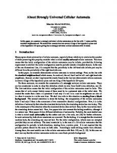
Given the fact that membership values, certainty factors and aggregation results are bounded in [0,1], if the hypothesis of the rule is not met at all, such a rule results to no change in the fuzzy set of the conclusion; it returns the initial membership value. On the other hand if the hypothesis is fully met and the rule‟s CF equals 1, it results to a fully urbanized cell. In any other case it returns a membership value within (m,1) where m is the initial membership value. CA are ideal simulators for the smooth urban expansion but they fail to simulate the spontaneous urbanization that occurs in detached areas. For this reason, following the paradigm of Geographic Automata Systems (Torrens 2003, Torrens & Benenson 2005), we added a third functional level that is triggered based on global rather than local attributes. These rules are triggered only in certain cells that have very high suitability values; otherwise they result to significant overestimation error. For this reason they use a specialized fuzzy hedge to limit the locations on which they are applied. “Top(a%) Fuzzy Hedge: Fuzzy Hedges within fuzzy systems play a role very similar to the role of numerical transformations in linear regression and usually correspond to raising the membership value to the power of some constant value. Our model incorporates a specialized hedge named “top(a%)” (Formula 5) which produces qualitative subsets of the original fuzzy membership function upon which it is applied. In example, “top(20%)” returns a full membership for all cells with an initial membership value μ of 0.8 or higher while it fades smoothly but very fast as μ diminishes. (5)

top.(a)  1

top.(a)  

if   1  a / 100 and 20(1   a / 100)

if   1  a / 100

Figure 3: the graph of the “top a%” fuzzy hedge shows its effect upon the initial membership value μ for different values of the α parameter.

10 4 CASE STUDY 4.1 The Area under Study The area under study is the broader area of Mesogia in east Attica in the mainland of Greece (Figure 4). The area’s surface is approximately 635 square km which for our case study is divided into 63.232 cells (100x100m). Broader Mesogia includes 18 municipalities in which more than 150.000 people find residence according to the 2001 census. It is particularly interesting to analyze urban growth and apply our model in this area for a number of reasons. To start with, the whole area lies within a distance of 10-25 km from the historical center of Athens but is separated by the main urban volume because of the particular geomorphology and specifically the mountain of Hemyttus. The east borders of the area are mapped out by the Aegean Sea while to the north and the south lies only a rather small amount of urban land cover. As a result the urban dynamics in the area may be considered relatively autonomous and can be studied separately from the neighboring areas. Mesogia composes an intricate land use mosaic including agricultural and natural lands with appealing conditions concerning the environment, the climate and the aesthetics only a few km away from the center of Athens which is the largest and most densely inhabited city of Greece. This is why during the last 20 years Mesogia has developed rapidly faster than any other area in Attica (Assimakopoulos et al., 2009). Specifically there were 60 square km of Urban Land Cover in 1994, 75 in 2000 and 125 in 2007. In other words, while Urban Land Cover grew by 25% during 1994-2000, it grew by 66% during 2000-2007. The significantly increased growth rate during the last decade is among others because of the new international airport, the extension of the Metro/train lines and a new highway network (Attiki Odos) and a number of sport facilities that were constructed in the area in the context of the development boost that was leveraged by the Athens 2004 Olympic Games. As a result, the city of Athens is expected to extend towards Mesogia. What is more, compared to the surrounding areas, Urban Land Cover is less homogenous presenting a more scattered spatial pattern. For all these reasons, the broader Mesogia area consists a proper yet challenging case to apply the model and evaluate its performance.

Figure 4: the location of the broader Mesogia area in east Attica in the mainland of Greece

11 4.2 Available Data and Pre-processing The list of available data includes:  Urban Land Cover for 2000 and 2007  Corine Land Cover (CLC) classification for 2000  Classified Road Network for 2000 and 2007  Subway and suburban train lines and stations  DEM Urban Land Cover data (30X30m) were previously produced based on Landsat images (Assimakopoulos et al., 2009) and were provided for the purpose of applying and testing the model. The Corine Land Cover database (100X100m spatial resolution) for 2000 is available from the European Environmental Agency and shows that most of the area is classified as Agricultural or Forest/Semi-natural while the vast majority of Artificial Surface is mainly Urban Fabric with the exception of the new airport. The road network was provided by Infocharta Ltd.2 for the years 2000 and 2007 and was classified in primary and secondary. For both road network classes for each year, two different layers were derived: density of the network in each cell and the minimum Euclidean distance of each cell from the network. Distance layers were also calculated from the main road network intersections and the subway/suburban train stations. The initial data for these features were also provided by Infocharta Ltd. Additionally, the DEM of the area that was acquired from the SRTM webpage3 (90X90m resolution) was used to produce a slope layer the spatial scale of which was changed to 100X100m. What is more, Urban Land Cover data were also converted to the same scale which at the same time allowed the production of fuzzy Urban Land Cover data through the application of the sum operator during the conversion. As a result, each of the 63232 cells of the areas under study were not binary described as urban or rural; instead for each cell the percentage of its surface occupied by Urban Land Cover was calculated. In example, a 100X100m. cell that overlays with 4 30X30 urban cells is assigned the value 40%. Finally all data combined into 2 combined raster data files (one for each year) whose spatial resolution is 100x100 m. and count 63232 cells each. These 2 files include all the necessary information to apply the model. 4.3 Rule’s Extraction for Suitability Calculator The file for the year 2000 was analyzed to extract the suitability rules for the same year. The Corine data were represented as singletons which means that each value (each land use type) was treated in separate without expecting similar values to present similar behavior. For each singleton, the percentage of overlapping between the singleton and the fuzzified Urban Land Cover data was calculated and used as the correspondent certainty factor. In example, in the area under study, approximately 65,2 sq.km were covered by complex cultivation patterns (class 242 according to the Corine classification) 14,3 of which appeared urban in the Urban Land Cover data. As a result the suitability for CLC 242 was calculated to be 22% (which is the division of 14,3 by 65,2) forming thus the following suitability rule: “If CLC in cell is 242, then the cell is suitable to support Urban Land Cover | CF=28%” The same procedure was applied for all land use types. A similar approach was followed for the rest quantitative data. Each value of each variable was treated as singleton for which the correspondent CF was calculated. The difference is that for each variable the full set of the couples variable value – correspondent CF was used 2 3

http://www.infocharta.gr/ http://www2.jpl.nasa.gov/srtm/

12 to form the membership function of each variable to the intermediate fuzzy set “suitable for Urban Land Cover”. In example, the distance of each cell from primary road network counts 1351 different values ranging from 0 m to 7400 for each one of which a CF was calculated defining thus a single point n a 2D space. The collection of these points can be visualized in a 2D graph which reveals the quantitative relation between the variable and the Urban Land Cover (Figure 5a). Analysis of the produced graphs allows us to extract exclusion rules. In example, CFs are zero or very close to zero for all slope values that are greater than 20 which leads to the crisp rule that excludes all such areas. Exclusion of cells decreases the number of cells that have a certain attribute (a certain land use or certain distance from a feature) but do not affect (in practice) the Urban Land Cover that is accumulated in these areas. This means that after the exclusion of areas, the CFs that were previously calculated tend to underestimate reality. For this reason, the procedure of KBE is repeated only for the dynamic (not excluded) cells which leads to updated graphs which present higher CFs (Figure 5b). Figure 6 shows the final graphs for all input variables.

Figure 5: a) the initial graph of CFs for the different slope values for the whole area (left) and b) the final graph after the exclusion of static areas (right).

Figure 6: the final CF graphs for (from left to right) Corine Land Cover, slope, , density of main road network, distance from main road network, density of secondary road network, distance from secondary road network, distance from main road intersections and distance from subway/suburban train stations. For the qualitative singleton data (CLC) the application of the calculated CFs is very easy since there is a single CF for each singleton (Table 1). Nevertheless, for the quantitative data, a numerical interpretation of the produced graphs is required for the purpose of the computational application. For this reason, interpolation between the local minimums and maximums of each graph was applied to produce a single numerical function that fits approximates the correspondent graph (table 2). These functions were used to calculate the CF of the quantitative suitability rules that have the following generic form: “If variable is x, then the cell is suitable to support Urban Land Cover | CF=f(x)”

13

CLC CF

111 0.60

112 0.62

121 0.25

133 0.11

222 0.20

223 0.10

242 0.22

243 0.10

Table 1: the correspondent CF for each Land use type singleton

Variable

Slope

CF function

μ(χ)=

{

μ(χ)=

{

Intersections distance (from)

μ(χ)=

{

Main road distance (from)

μ(χ)=

Main road density

Stations distance (from)

if χ  [0,2] if χ  (2,8) if χ  [8,21]

0.25 0.25(11 - χ)/9 0.25(21 - χ)/39

0.58 [(χ  500)/1500] 0.58(2500 - χ)/1500 0

0.5

if χ  [0,1000] if χ  (1000,2500) else

0.30 [(2500 - χ)/2000] 0.66 0

if χ  [0,500] if χ  (500,2500) else

{

0.45exp( - χ / 360 ) 0

if χ  [0,3000] else

μ(χ)=

{

0.01 χ 1

if χ  100 else

Secondary road distance (from)

μ(χ)=

{

0.40 exp( - χ / 100) 0

If χ  [0,2000] else

Secondary road density

μ(χ)=

{

χ / 80 1

if χ  80 else

0.30

Table 2: the correspondent CF function for each quantitative input variablee

14 4.4 Calibration The suitability rules that were extracted (as described in the previous subsection) are applied in the Suitability calculator which uses exclusively the Sensitive Sum operator. The result is the intermediate thematic layer that maps the overall suitability of each cell to support urban land cover (Figure 7b). The suitability layer calculation is an entirely independent process from simulation. This fact, along with the parallel rules‟ connection that SS implements, allows us to add any data that might be available in order to update the Suitability Layer without altering the knowledge that was extracted for the initial data or the simulation mechanism. Once the overall suitability layer is calculated the model is calibrated manually through trial and error test. More specifically, the parameters that are subjected to calibration are the CFs and the radiuses of the Moore neighborhoods used in each one of the three functions of the Simulator (intensification, edge expansion and spontaneous growth) and the a parameter of the fuzzy hedge “top(a%)” that is applied in the spontaneous growth function. Manual calibration suggested that:  The intensification function operates upon a 3X3 neighborhood with a 0.8 CF  The edge expansion function operates upon a 5X5 neighborhood with a 0.9 CF  The spontaneous growth function applies a 0.8 CF upon cells that have a suitability value greater than 60% and are located 500m away or more from existing urban land cover. The initial configuration appeared to underestimate the urban density of the Northwest part of the area and the spatial extend of urban cover in the South-east part. For this reason the CF of the CLC class 222 was increased by 50% while the CF function of the main road density received a 20% boost in the South-east area (without exceeding 100% though in any case). Additionally, the intensification function was allowed to operate upon 5X5 Moore neighborhoods in the North-west area. 4.5 Results and Evaluation In order to calibrate and evaluate the model, objective indicators are required that assess the fitting of the model’s results to reality. For this reason, the model calculates three fitting indicators between the results and the actual urban land cover when available:  the Lee-Sallee statistic which shows how correctly coincident are the results of modeling with the spatial shape of the actual urban area (Kim et al., 2006). Its values range from 0, indicating no coincidence, to 1, indicating a perfect coincidence.  the K coefficient of agreement which expresses the agreement between two categorical datasets, corrected for the agreement as can be expected by chance, which depends on the distribution of class sizes in both datasets (Bishop et al., 1975). Kappa is well suited to compare a pair of land use maps with its values ranging from 1, indicating a perfect agreement, to -1 indicating no agreement (Jasper, 2009).  the K-simulation index of agreement which is an adjusted K coefficient that takes into consideration not only the fitting of the results to the actual urban cover, but also the fitting between the initial and the final point (Jasper, 2009)  the average error per 5x5 neighborhoods, this index allows overestimation and underestimation errors that occur within 500m. to neutralize each other. The model was applied on data referring to the year 2000 and attempted to produce an estimation of the 2007 urban land cover. This is a rather short period; nevertheless, urban land cover in 2007 (Figure 7c) is 66% (according to the data used) more than urban land cover in 2000 (figure 7a) while in most cases studied urban growth is approximately 10% (Pontius & Malanson, 2005) which makes our case a challenging one. The fitting indicators (Table 3) of the model’s results (Figure 7d) to the actual 2007 urban land cover estimate imply that the models produces rather satisfactory estimations, at

15 least for the specific case. More specifically, the Lee-Sallee statistic suggests that the spatial overlapping of the actual and the estimated urban land cover exceeds 70% while Kappa index indicates an 80% agreement between the values of actual and the estimated urban land cover. The K-simulation index on the other hand, suggests that only 45% of the actual growth that occurred is accurately estimated. Nevertheless, this does not imply any deficiency that is attributable to the model itself, since the K-simulation has only recently been proposed and has not yet been widely applied. As a result, we cannot compare it with other applications. Finally, the average error calculated in 5X5 Moore neighborhoods suggests that only 6% of the results fail to capture the actual urban land cover in a coarser spatial scale.

Figure 7: a) actual urban land cover in 2000 (top left), b) suitability to support urban land cover calculated using data for 2000 (top right), c) actual urban cover in 2007 (bottom left) and c) estimation of the 2007 urban land cover using data for 2000 (bottom right). LeeShalle 0.71

K 0.80

Ksim 0.45

Moore5 0.06

Table 3: the values of the fitting indicators of the model’s results to real urban land cover.

16 The fitting indicators suggest that the model can be used to produce short-term estimations of the future urban land cover for the specific area under study. This allows us to apply the KBE procedure that was described previously on 2007 data and calculate the suitability to support urban land cover for the same year. In turn, this enables the application of the urban simulator – without additional calibration though – and the population of urban growth scenarios for the Mesogia area until at least 2014. Specifically, two different scenarios were populated, one assuming a 30% growth (Figure 8a) and one assuming a 50% growth (Figure 8b) respectively. The two scenarios do not differ significantly concerning the spatial extend of urban land cover but they do present significant differences in the local values of urban land cover density values. Both scenarios suggest that almost all areas that are accessible through road network will become urban putting in danger most agricultural activities in Mesogia which until 2000 was primarily rural.

Figure 8: a) the 30% urban land cover growth (left) and b) the 50% urban land cover growth for the same year (right).

5 CONCLUSIONS AND FUTURE DEVELOPMENTS The model presented in this paper utilizes Fuzzy Algebra to map the effect of any spatial or spatially referenced variable to the urban growth occurred in an area without requiring certain data or certain spatial resolution of data in order to run. For this reason, the model can be easily transferred to both data rich and data poor cases. The separate effects of different input variables are merged in a single Suitability layer by the Suitability calculator component which utilizes exclusively the Sensitive Sum operator. SS applies a parallel connection to each effect taking into account the correlation between them; presenting thus all advantages of the probabilistic sum operator while eliminating the tendency to overestimate values. This way, not only knowledge base sustains a reducible/extensible form but also using a large number of input variables does not result to highly complex analysis. Fuzzy logic is an advisable framework to deal with vague data and provides the proper tools for the management of uncertainty. It allows the process of information in a hybrid qualitative/quantitative way and expresses the dynamic of the phenomenon under study in common linguistic terms. The rules syntax is kept simple and hence comprehensible; as a result the user can easily add empirical rules to the data-driven ones and experiment In order to simulate urban growth, Cellular Automata techniques that use either linear or exponential transition functions are incorporated while pseudo-agent behavior is also added. Using exponential transition does not alter the spatial extend of the outcomes but improves the numerical fitting to the actual urban cover. Linear CA manage the rural-urban transition for

17 cells that are in the vicinity of existing urban land cover, while pseudo agent rules allow the rural-urban transition to take place in cells that are detached from the main urban land cover and have a very high suitability. The model was calibrated and applied in the Mesogia area in east Attica for the period 2000-2007 during which urban land cover grew by 66%., consisting thus a challenging case. Nevertheless, the models produces a rather satisfactory estimation of the 2007 urban land cover as implied by the fitting indicators calculated. On top of this, part of the error cannot be avoided because of the rather small amount of available data that cannot diversify easily which cells present higher suitability than others. The small amount of data and more specifically the fact that data were available for only two times, narrows the significance of the results. Ideally, data for two different periods – one to calibrate and one to test the model - would allow a significantly more trustworthy evaluation of the behavior of the model. This is the first direction towards which future work is planned. Along with this, it is also very important to apply the model in other areas as well which will reveal whether the model can be equally efficient. From a technical point of view, an automated calibration module should be developed to introduce spatial variability and temporal variability if sufficient data are available while a number of potential improvements can be made, possibly by employing directional CA. Acknowledgements. The research leading to these results has received funding from the European Community's Seventh Framework Programme FP7/2007-2013 under grant agreement n° 212034

BIBLIOGRAPHY Assimakopoulos, D., Petrakis, M., Chrysoulakis, N., Stathopoulou, M., Karvounis, G., C. Cartalis, 2009, Olympic Games in Athens: using earth observation for the assessment of changes and impacts for the natural and built environment. Annual Dragon 2 Symposium, Barcelona,Spain, June 22 – 26, Barredo J., Kasanko M., McCormick N., Lavalle C., 2003, Modeling dynamic spatial processes: simulation of urban future scenarios through cellular automata, Landscape and Urban Planning, vol.64, p.145-160, Benenson I., Kharbash V., 2006, Geographic Automata Systems and the OBEUS Software for their Implementation, Complex Artificial Environments, Springer Berlin Heidelberg, p.137-153, Blecic Ι., Cecchini A., Prastacos P., Trunfio G.A., Verigos E., 2004, Modelling Urban Dynamics with Cellular Automata: A Model of the City of Heraclion. 7th AGILE Conference on Geographic Information Science, University of Crete Press, Heraklion, Greece, Bishop Y. M. M., Fienberg S.E., Holland P.W., 1975, Agreement as a special case of association. Discrete Multivariate analysis. Cambridge MA, MIT press, p.393 – 400. Chen M.Y., Linkens D.A., 2004, Rule-base self-generation and simplification for data-driven fuzzy models, Fuzzy Sets and Systems, vol.142, p.243-265, Cheng J., Masser, I., 2003, Understanding Urban Growth System: Theories and Methods. 8th International Conference on Computers in Urban Planning and Urban Management, Sendai City, Japan, Chrysoulakis N., Kamarianakis Y., Farsari Y., Diamandakis M., Prastacos P., 2004, Combining Satellite And Socioeconomic Data For Land Use Models Estimation, EARSeL Workshop on Remote Sensing for Developing Countries, Cairo,

18 Corgne S., Hubert-Moy L., Dezert J., Mercier G., 2003, Land Cover Change Prediction With A New Theory Of Plausible And Paradoxical Reasoning, 6th International Conference of Information Fusion, Caimes, Queensland, Australia, Dietzel Ch., Clarke K. C., 2004, Replication of Spatio-Temporal Land Use Patterns at three Levels of Aggregation by an Urban Cellular Automata. Lecture Notes in Computer Science, vol. 3305, p. 523-532, Dietzel Ch., Oguz H., Hemphill J. J., Clarke K. C., Gazulis N., 2005, Diffusion and Coalescence of the Houston Metropolitan Area: Evidence Supporting a New Urban Theory, Environment and Planning B: Planning and Design, vol.32, p.231-246, Dragicevic S., 2004, Coupling Fuzzy Sets Theory and GIS-based Cellular Automata for LandUse Change Modeling, In Fuzzy Information, IEEE Annual Meeting of the Processing NAFIPS'04, Banff, Canada, vol.1, P.203-207, Hagen-Zanker A., Van Loon J., Straatman B., De Nijs T., Engelen G., 2005, An Evaluation Framework for the Calibration and Validation of Integrated Land Use Models Featuring Cellular Automata, 14th European Colloquium on Theoretical and Quantitative Geography, Tomar, Portugal, Hagoort M., Geertman S., Ottens H., 2008, Spatial Externalities, Neighbourhood Rules And CA Land-Use Modelling, The Annals of Regional Science, vol.42, no.1, p.39-56, Hatzichristos Th., 2001, GIS and Fuzzy Logic in Spatial Analysis. Educational notes, NTUA, Heikkila E. J., Shen T.Y., Yang K.Z., 2002, Fuzzy Urban Sets Theory and Application to Desakota Regions in China, Environment & Planning B: Planning and Design, vol. 29, p.239-254, Jasper V., 2009, Assessing the Accuracy of Changes in Spatial Explicit Land Use Change Models, 12th AGILE International Conference on Geographic Information Science 2009, Hannover, Germany Kim J., Kang Y., Hong S., Park S., 2006, Extraction of Spatial Rules using a Decision Tree Method: A Case Study in Urban Modeling. In Gabrys B., Howlett R. J., Jain L. C. (Eds.), KES 2006, Part I, LNAI 4251 (pp. 203 – 211), Springer-Verlag Berlin Heidelberg Kirschfink H., Lieven K., 1999, Basic Tools for Fuzzy Modeling, Tutorial on Intelligent Traffic Management Models in Helsinki, Klopotek M.A., Wierzchon S.T., 2000, Empirical Models for the Dempster-Shafer Theory, Belief Functions in Business Decisions, p.62-112, Koutsopoulos K., 2002, Geographic Information Systems and Spatial Analysis, Papasotiriou, Krawczyk R.J., 2003, Architectural Interpretation of Cellular Automata, Poster presented at NKS 2003, Boston, Liu Y., Phinn S.R., 2001, Developing a Cellular Automaton Model of Urban Growth Incorporating Fuzzy Set Approaches. Proceedings of the 6th International Conference on GeoComputation, University of Queensland, Brisbane, Australia, Liu Y., Phinn S.R., 2003, Modelling Urban Development With Cellular Automata Incorporating Fuzzy-Set Approaches, Computers, Environment and Urban Systems, vol.27, p.637-658, Malczewski J., 2004, GIS-Based Land-Use Suitability Analysis: A Critical Overview, Progress in Planning, vol.62, p.3-65, Miranda V, Monteiro C., 1999, Fuzzy Inference Applied to Spatial Load Forecasting, Power Tech ’99 Conference, Budapest, Hungary, Morshed A., 2002, Land Use Change Dynamics: a Dynamic Spatial Simulation. PhD Thesis, Mraz M., Zimic N., 1999, Intelligent bush fire spread prediction using fuzzy cellular automata, Journal of Intelligent and Fuzzy Systems, vol.7, p.203-207, Mulianat I., Hariadi Y., 2004, Urban Area Development in Stochastic Cellular Automata, Urban/Regional, EconWPA,

19 Ness G. D., Low M. M., 2000, Five Cities: Modelling Asian Urban Population-Environment Dynamics, Oxford University Press, p.43-67, Packard N. H., Wolfram S., 1985, Two-Dimensional Cellular Automata, Journal of Statistical Physics, vol.32, no.5/6, p.901-946, Pontius G. R., Malanson J., 2005, „Comparison of the structure and accuracy of two land change models‟, International Journal of Geographical Information Science, ωολ.19, νο.2, p.243-265 Sasikala K. R., Petrou M., 2001, Generalised Fuzzy Aggregation in Estimating the Risk of Desertification of a Burned Forest, Fuzzy Sets and Systems, vol.118, no.1, p.121-137, Setnes M., Babuska R., Verbruggen H. B., 1998, Transparent Fuzzy Modelling, Human & Computer Studies, vol.49, p.159-179 Torrens, P. M., 2003, Automata Based Models Of Urban Systems, Advanced Spatial Analysis, ch.4, p.61-79, Torrens P.M., Benenson I., 2005, Geographic Automata Systems, Geographical Information Science, vol. 19, no.4, p.385–412, Vancheri Α., Giordano P., Andrey D., Albeverio S., 2004, A Model for Urban Growth Processes with Continuum State Cellular Automata and related Differential Equations, Witlox F., Derudder B., 2005, Spatial Decision-Making Using Fuzzy Decision Tables: Theory, Application and Limitations, Fuzzy Modeling with Spatial Information for Geographic Problems, p.253-274, Wolfram S., 1984, Cellular Automata as Models of Complexity, Nature, vol.311, p.419-424, Wu F., 1996, A Linguistic Cellular Automata Simulation Approach for Sustainable Land Development in a Fast Growing Region, Computer, Environment and Urban Systems, vol.20, no.6, p.367-387, Wu F., 1998, Simulating Urban Encroachment On Rural Land With Fuzzy-Logic-Controlled Cellular Automata In A Geographical Information System, Journal of Environmental Management, vol.53, p.293-308 Wu F., 2002, Calibration of Stochastic Cellular Automata: the Application to Rural-Urban Land Conversions, Geographical Information Science, vol.16, no.8, p.795–818, Yeh A. G.O., Li X., 2003, Error Propagation and Model Uncertainties of Cellular Automata in Urban Simulation with GIS, 7th International Conference on GeoComputation University of Southampton, United Kingdom, Zadeh L. A., 1965, Fuzzy Sets, Information and Control, no.8, p.338-353, Zadeh L. A., 1993, Fuzzy Logic, Journal of Intelligent Information Systems, vol.2, p.309-310, Zadeh A. L., 2006, Generalized Theory of Uncertainty (GTU), Principal Concepts and Ideas Advances in Soft Computing, p.3-4