I. H. Altas and J. Neyens, A Fuzzy Logic Load-Frequency Controller for Power Systems, International Symposium on Mathematical Methods in Engineering, MME-06, Cankaya University\ Ankara, Turkey, April 27 - 29 , 2006.
A Fuzzy Logic Load-Frequency Controller for Power Systems İsmail H. Altaş1 and Jelle Neyens2 1
Department Of Electrical and Electronics Engineering, Karadeniz Technical University, Trabzon, Turkey
[email protected]
2
Department Electrical energy, Systems & Automation, Gent university, Gent, Belgium
[email protected]
Abstract — A fuzzy logic based load frequency controller model for power systems is developed and simulated in this paper. The proposed simulation model is compared with the classical regulating systems in order to verify and show the advantages of the model and controller developed. The design process of the proposed fuzzy logic controller is given in detail step by step to show a direct and simple approach for designing fuzzy logic controllers in power systems.
1 Introduction Load-Frequency (L-F) control is an important task in electrical power system design and operation. Since the load demand varies without any prior schedule, the power generation is expected to overcome these variations without any voltage and frequency instabilities. Therefore voltage and frequency controllers are required to maintain the generated power quality in order to supply constant voltage and frequency to the utility grid. The frequency control is done by load-frequency controllers, which deals with the control of generator loadings depending on the frequency. Many research has been done and different approaches has been proposed over the past decades regarding the load-frequency control of single and multi area power systems [1-12]. The main purpose of designing load-frequency controllers is to ensure the stable and reliable operation of power systems. Since the components of a power system are non linear, a linearized model around an operating point is used in the design process of L-F controllers. Some of the proposed methods in literature deal with system stability using fixed local plant models ignoring the changes on some system parameters [8-12]. Fuzzy set theory provides a methodology that allows modeling of the systems that are too complex or not well defined by mathematical formulation. Fuzzy logic controllers based on fuzzy set theory are used to represent the experience and knowledge of a human operator in terms of linguistic variables that are called fuzzy rules. Since an experienced human operator adjusts the system inputs to get a desired output by just looking at the
ALTAŞ, NEYENS system output without any knowledge on the system’s dynamics and interior parameter variations, the implementation of linguistic fuzzy rules based on the procedures done by human operators does not also require a mathematical model of the system. Therefore a fuzzy logic controller (FLC) becomes nonlinear and adaptive in nature having a robust performance under parameter variations with the ability to get desired control actions for complex, uncertain, and nonlinear systems without the requirement of their mathematical models and parameter estimation. Fuzzy logic based controllers provide a mathematical foundation for approximate reasoning, which has been proven to be very successful in a variety of applications [10]. As in many different areas, the use of fuzzy logic controller has been increased rapidly in power systems, such as in load-frequency control, bus bar voltage regulation, stability, load estimation, power flow analysis, parameter estimation, protection systems, and many other fields. Fuzzy logic applications in power systems are given in [8] with a detailed survey. Any load change in one of the L-F control areas affect the tie line power flow causing other L-F control areas to generate the required power to damp the power and frequency oscillations. The response time of the L-F controllers is very important to have the power system to gain control with increased stability margins. Therefore the proposed L-F controller must reduce the response time as well as reducing the magnitude of the oscillations when compared to that of classical types. The results of the classical controller and the fuzzy logic controller are compared, and since the response time of the stabilizer of the load frequency is very important, a quicker an more stable solution is achieved with FL controller than the one found by controlling in a classical way
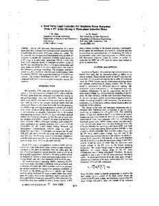
2 The Load-Frequency (L-F) Control The principle block of the power system studied in this paper is given in Figure 1. Two parts of this system can be considered. A considerable attention should be pay to the LFC (Load Frequency Control) section. Changes in real power mainly affect the system frequency, while reactive power is less sensitive to changes in frequency and is mainly dependent on changes in voltage magnitude. The LFC thus controls the real power and the frequency of the system. It also has a major role in the interconnection of different power plants [6]. The LFC is used to maintain a reasonable uniform frequency. The first step of control engineering consists of mathematical modeling. Two methods are well-known: the transfer function method and the steady state method. Linear systems can not often be found in real situations, but a close approximation by linearizing is suitable for simulation. A simulation model derived here using the transfer function model [6]. The block diagram that represents the approximation of the real system behaviors is shown in Figure 2. This is a small signal model used to represent the influence of load changes. The source of mechanical power, commonly known as the prime mover, may be either hydraulic energy or steam. The mathematical model for the turbine relates the changes in mechanical power output ∆Pm to changes in steam valve position ∆PV. Both ∆Pm and ∆PV are represented by x2 and x1, respectively, in Figure 2. The most simple prime mover model can be approximated with a single time constant such as the one given by τg in Figure 2 where the variables x1, x2, x3 and x4 are equal to ∆PV, ∆Pm, ∆ω and output of the
A FUZZY LOGIC LOAD-FREQUENCY CONTROLLER FOR POWER SYSTEMS integral controller signal, respectively. The steady state equations can be drawn from the simulation diagram easily as in Equation (1). Water or steam input
vfs
Controlled gate
Substation
GOV
∆ω
vt a
vLL
ω
-
Transmission lines
GENERATOR
EXCITER
Turbine
Rectifier
∆ vt AVR
+
+
ω ref
- vt
Power grid
vref
Figure 1. Control block diagram of the power system. 1 τg
+ -
1 s
x1 + x3
1 R
1 τT
1 s
1 x2 s
1 2H
-
+ -
Ki
x4
1 s
+
-
PL impulse
D plot
Figure 2. Simulation block diagram of a single area power system with an integral controller. ⎡ 1 ⎢− ⎡ x&1 ⎤ ⎢ τ g ⎢ x& ⎥ ⎢ 1 ⎢ 2⎥ = ⎢ ⎢ x&3 ⎥ ⎢ τ T ⎢ ⎥ ⎢ 0 ⎣ x& 4 ⎦ ⎢ ⎣⎢ 0
0 −
−
1
0
τT
1 2H 0
1 τgR
−
D 2H KI
−
1⎤ τ g ⎥ ⎡ x1 ⎤ ⎡ 0 ⎤ ⎥ ⎥ ⎢ ⎥ ⎢ 0 ⎥ ⎢ x2 ⎥ + ⎢ 0 ⎥ ∆P 1 ⎥ ⎥ ⎢ x3 ⎥ ⎢⎢− 2 H ⎥⎥ 0 ⎥ ⎢⎣ x4 ⎥⎦ ⎢⎣ 0 ⎥⎦ ⎥ 0 ⎥⎦
(1)
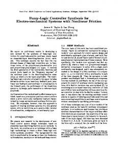
3 Fuzzy Logic Controller As explained in the introduction, the FLC performs the same actions as a human operator by adjusting the input variables, only looking at the system output. The controller consists of three sections: fuzzifier, rule base and defuzzifier, as shown in Figure 3. The fuzzifier first converts its two input signals, the main signal (∆ω in this case), and the step change of every sample ∆(∆ω), to fuzzy numbers. This numbers are the input of the rule table, which calculates the fuzzy-number of the controlled output signal by taking the right decisions. Finally this resulting number is converted in the defuzzifier to the crisp values.
ALTAŞ, NEYENS
Defuzzifier
Fuzzifier
Fuzzy Inference System As the classical controller the FLC also ∆P(k-1) ∆ω(k) has an integrating part to be implemented. ∆(∆ P(k)) + Therefore the controller has to be designed + ∆(∆ω(k)) Rule + in such a way that the resultant increBase mental output ∆(∆P(k)) is added to the ∆ω(k−1) ∆P(k) previous value ∆(∆P(k-1) to yield the current output ∆(∆P(k). It should be noted Figure 3. Basic structure of fuzzy logic that this is nothing but the digital implecontroller. mentation of an integrator, using Euler integration. The FL rules in the FLC are developed to yield a similar but more effective output than an integrator gives. The difference between a fuzzy logic controller and an integral controller is the procedure used to calculate ∆(∆P(k)).
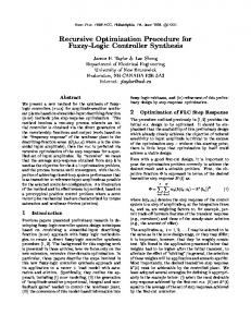
3.1 Fuzzy Inference System Figure 3, there are two inputs to the fuzzy inference system. The first one is the change in angular velocity, the other one is the change of it ∆(∆ω(k)). As we want the angular velocity to be constant, the change of this velocity can be considered as the disturbance of the system, and should be reduced to zero as soon as possible. These two inputs are fuzzified and converted to fuzzy membership values that are used in the rule base in order to execute the related rules so that an output can be generated. The fuzzy rule base, or the fuzzy decision table, is the unit mapping two crisp inputs, the just mentioned ones, to the fuzzy output space defined on the universe of ∆(∆P(k)). To simplify the following text, the iteration counter will be omitted from now on. The time response of the disturbed change in angular velocity for an impulse input can be represented by the generalized impulse response error of a second order system. We are interested in the impulse response for the reason that when a uniform step in the angular velocity, ω, appears, the derivative of ω will be one, and zero at any other time. Since the intention is to design a fuzzy logic controller with a better performance (shorter settling time, less over-shoot) than the classical controller, the response signal of this system can be taken as a reference to construct the rule table on. The impulse response of the system generated without any controller is given in Figure 4. This response is used to represent the operational behavior of frequency changes in a single area power system in order to generate fuzzy rules. The fuzzy rules represent the knowledge and abilities of a human operator who makes necessary adjustments to operate the system with minimum error and fast response. It is necessary to observe the behaviors of the error signal ∆ω and its ∆(∆ω)on different operating regions in order to model the actions a human operator would take, in every different case, deciding whether the change, ∆(∆P), in the controller output should be increased or decreased according to the inputs of the fuzzifier. This controlled output is the required change in the input of the system. The derivative of the impulse response signal of the system without ant controller is shown in Figure 5. As been told, the results shown in both Figure 4 and 5 can be useful to construct the rule table. The values we read on this graphics will be used to define the first fuzzy set intervals. By applying trial-and-error in order to achieve improved results with the FLC, these intervals may change.
A FUZZY LOGIC LOAD-FREQUENCY CONTROLLER FOR POWER SYSTEMS 4
x 10
-4
x 10
-5
1
Change in frequency (pu)
Change in Frequency (pu)
2 0 -2 -4 -6 -8 -10
0.5 0 -0.5 -1 -1.5
0
2
4
6
Time (sec.)
8
10
-2
1
2
3
4
5
6
7
8
9
Time (sec.)
Figure 4. Impuls response of the system with- Figure 5 Classical controller impuls response out any controller signal's derivative.
We first try to develop an initial rule base (with only 3 fuzzy sets), which we will extend to a 5 fuzzy sets base. According to the signs of ∆ω and ∆(∆ω), we decide whether the sign of ∆(∆P) has to be positive or negative. A summary of all possible situations, or so called operation regions, is given in Table 1. ∆ω ∆(∆ω) ∆(∆P)
+ +
Operating Regions 0 - - 0 + - + 0 - - + + + 0 0 0 - - - + + - + 0
Table 1. Output decision making table. The sign of ∆(∆P) should be positive if ∆P has to be increased and it should be negative otherwise. This simple rule is applied as in Table 1 to determine the sign of ∆(∆P). A verbal example of these rules is: “The error is positive and decreasing towards zero. Therefore, ∆(∆P) is set to positive to reduce the error.” This example expresses the first column of Table 1. Similar reasoning can be applied for the other columns. A 'programming language translation' of this table gives: IF∆ω is zero THEN ∆(∆P) takes the sign of ∆(∆ω) ELSE IF ∆(∆P) takes the sign of ∆ω.
(2)
Table 1 shows that each one of ∆ω, ∆(∆ω) and ∆(∆P) has three different options for the signs to be assigned. They are either positive, negative or zero. With this knowledge, an initial rule decision table with twenty five rules can be formed like in Table 2, whwre 'N' means negative, 'O' zero and 'P' positive. The main part without shading represents the rules as well as the signs of ∆(∆P). From this table on, some logical reasoning should be considered. A closer look at Table 2 shows that in some cases, there is a transition from negative to positive, without passing zero. Therefore, an adjustment in the initial rule table leads to another table without this inconvenience. The influence of ∆(∆ω) must stay, and a symmetric solution has to be advised, so the modified rule table is the one that can be found as in Table 3.
ALTAŞ, NEYENS M N 0 P Q ∆(∆ω)
M N N N N 0
N N N N 0 P
0 N N 0 P P
P N 0 P P P
Q 0 0 P P P
∆ω
∆(∆P) Table 2. Initial rule table.
M N 0 P Q ∆(∆ω)
M M M N N 0
N M N N 0 P
0 N N 0 P P
P N 0 P P Q
Q 0 0 P Q Q
∆ω
∆(∆P) Table 3. Modified rule table.
10
0
-1
-2
M
N
0
P
1
Q
-4
∆ω
µ(∆(∆ω))
In Table 3, a slightly different meaning of the applied letters is used: 'M' means large negative, 'N' small negative, 'O' stays zero, 'P' becomes small positive and 'Q' large positive. Now the output values of ∆(∆P) are extended to five regions as it is done for input spaces. This rule table is the final one; the one that's going to be used in the FLC. As suggested, the initial limits of the fuzzy Q M 0 N P sets will be derived from the diagram obtained by using the classical controller. The set values can be derived immediately ∆(∆ω) from Figures 4 and 5; but a plot of ∆ω versus ∆(∆ω) is preferred. The fuzzy sets consist of triangular functions. A visualization of the definition of these fuzzy sets can be seen on Figure 6. In this case, the scaling of the fuzzy sets representing the partitioning will be different for ∆ω and ∆(∆ω). As shown in Figure 6, the interval 2 -1 3 -6 0 1 of the latter is much smaller yielding diffeµ(∆ω) 10 rent scaling for a proper operation of the controller. The fuzzy sets will initially be Figure 6. Partitioning input spaces into five regions. defined in the interval [−1.5 ×10 −4 ,−1.5 ×10 −4 ]
for ∆ω, and [−1.5 ×10 −6 ,−1.5 ×10 −6 ]
for ∆(∆ω)
(3)
The combination of Table 3 and Figure 6 gives a well defined summary of the fuzzy sets and the rules that should be applied on those. The next step in the design process is the fuzzy reasoning as discussed below.
A FUZZY LOGIC LOAD-FREQUENCY CONTROLLER FOR POWER SYSTEMS 3.2 Fuzzy Reasoning The crisp universes of ∆ω, ∆(∆ω) and ∆(∆P) have been partitioned into five regions as M, N, O, P and Q as explained earlier. These five regions in all three universes are represented by triangular fuzzy membership functions defined by (4) and shown in Figure 7 where ‘b’ is the crisp value with a membership degree of 1 in the corresponding fuzzy set. 'a' and 'c' define the limits of the triangular fuzzy set (symmetric in this paper.)
⎡
⎛ x−a c−x⎞ ⎤ , ⎟,0⎥ ⎝ b−a c−b ⎠ ⎦
µ ( x) = max ⎢min⎜ ⎣
(4)
The universe of , b=-1.5×10⁻⁴ for M, b=-0.75×10⁻⁴ for N, b=0 for O, b=0.75×10⁻⁴ -4 for P, b=1.5×10 for Q. A similar, equal-regions and symmetric partition is made for the universes of ∆(∆ω) and ∆(∆P). In addition to the definition of these triangular functions, it is required to calculate the membership degree of ∆(∆P), as well. The following example is given to clarify the method used to obtain the membership values in output space. When ∆ω=0.45×10⁻⁴ it intercepts with the fuzzy sets N and O in the input universe of ∆ω, and when ∆(∆ω)=0.15×10⁻⁴ it intercepts with the fuzzy sets O and P in the input universe of ∆(∆ω) as shown in Figure 8 which is a close-up of the fuzzy-sets of Figure 6. µ(x)
µ(x)
1.0 µ3=0.6667
1.0
N
0
P
µ1=0.6
µ(x(k))
µ2=0.4 µ4=0.3333
a
x(k) b
c
Figure 7. Triangular fuzzy membership function.
∆ω=0.45x10⁻⁴
-6
∆(∆ω)=0.15x10
Figure 8. Snapshot of the process at a certain time.
The membership degrees of all fuzzy triangular functions can easily be found by applying formula (4), in which we substitute a, b and c by the appropriate limits; x takes the value of either ∆ω or ∆(∆ω). The horizontal lines drawn through the intercepting points of ∆ω on N and O in Figure 8 gives the membership values of ∆ω on N and O, respectively, while the horizontal line passing through the intercepting points of ∆(∆ω) and O and P gives the membership values of ∆(∆ω) on these fuzzy sets, respectively. These membership values of ∆ω and ∆(∆ω) on N, O, O and P are evaluated by Table 3 to yield the fuzzy membership values of the following active rules at the output space. R1: If ∆ω R2: If ∆ω R3: If ∆ω R4: If ∆ω
is N and ∆(∆ω) is O then ∆(∆P) is N is N and ∆(∆ω) is P then ∆(∆P) is O is O and ∆(∆ω) is 0 then ∆(∆P) is O is O and ∆(∆ω) is P then ∆(∆P) is P
ALTAŞ, NEYENS The application of the min-operator results in the following membership values from each active rule to be used in the output space ∆(∆P). µ R1 (∆(∆P)) = min(µ N (∆ω ), µ O (∆(∆ω ))) = min(0.63,0.67 ) = 0.63 µ R 2 (∆(∆P)) = min (µ N (∆ω ), µ P (∆(∆ω )) ) = min (0.63,0.33) = 0.33 µ R3 (∆(∆P)) = min(µO (∆ω ), µO (∆(∆ω )) ) = min(0.40,0.67 ) = 0.40 µ R 4 (∆(∆P)) = min(µO (∆ω ), µ P (∆(∆ω ))) = min(0.40,0.33) = 0.33
These resultant membership values of the active rules determine the weights of the fuzzy sets in the universe of ∆(∆P). The average of these membership values, multiplicated with the crisp value corresponding with the respective fuzzy set, is used to obtain final crisp output as ∆(∆P(k)). This final process is called defuzzification of the fuzzy output. Several defuzzification methods have been applied in literature. However, the method, called 'the center of area' is widely used in fuzzy logic control applications. The method can be implemented as follow using the data of the example given. 4
∑ µ Ri (∆(∆P)).(∆(∆P)i
∆(∆P (k ) ) = i =1
(5)
4
∑ µ Ri (∆(∆P)) i =1
∆(∆P(k ) ) =
(0.63)(−0.5) + (0.33)(0) + (0.4)(0) + (0.33)(0.5) − 0.15 = = −0.08876 0.63 + 0.33 + 0.4 + 0.33 1.69
4 L-F Control with Fuzzy Logic The FL controller is placed on the path where the frequency variation, ∆ω, is fed back governor in power system as shown in Figure 9. The steady state matrices for the FLC can be constructed using Figure 9. + -
1 τg
1 s
x1 + x3
1 R
1 τT
1 s
1 x2 s
+
1 2H
-
Fuzzy Logic Controller
d dt
+
-
PL impulse
D plot
Figure 9 The block diagram of the FL controlled L-F scheme.
A FUZZY LOGIC LOAD-FREQUENCY CONTROLLER FOR POWER SYSTEMS Figure 9is the main simulation diagram of the L-F control scheme to be used with FL controller. As it can be seen from the fact that the system has third order equations with FLC instead of four as it is the case with classical integrator. From Figure 9, the steady state equations can be composed as in (6) where x1=∆Pv, x2=∆Pm and x3=∆ω. ⎡ 1 ⎢− τ & ⎡ x1 ⎤ ⎢ g ⎢ x& ⎥ = ⎢ 1 ⎢ 2⎥ ⎢ τ ⎢⎣ x&3 ⎥⎦ ⎢ T ⎢ 0 ⎢⎣
0 −
1
τT
1 2H
⎡ 1 ⎤ ⎢ ⎥ τgR x ⎥⎡ 1 ⎤ ⎢ ⎢ 0 ⎥ ⎢⎢ x2 ⎥⎥ + ⎢ ⎥ ⎢ ⎥ ⎢ D ⎥⎥ ⎣ x3 ⎦ ⎢ − ⎢ 2 H ⎥⎦ ⎣
−
⎤ 0 ⎥ ⎥ ⎥ ⎡ du ⎤ 0 ⎥⎢ ⎥ ⎥ ⎣∆PL ⎦ 1 ⎥ − 2 H ⎥⎦
1
τg 0 0
(6)
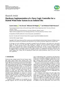
5 Results Both of the systems, L-F control with classical integral and fuzzy controller, will be simulated using the parameter values as τ t = 0.5, τ g = 0.2, H = 5, D = 0.8, R = 0.05, K i = 7, ∆PL = 0.2 The resultant graph of the classical system is already shown in Figure 4. The results obtained by the fuzzy logic controlled system are shown in Figure 10. Both graphics have the same steady state results: zero. On this point, no improvements can be made. Nevertheless the settling time and the overshoot can be adjusted. First a plot of the impulse response is obtained as given in Figure 10, while the intervals of the fuzzy sets are those described and derived from the results of the classical controller given by equation (6). As expected, the response of the fuzzy logic system with the initial intervals gives similar results as the classical system. Although, some damping effects with longer settling time can also be observed from the response given in Figure 11. By making some adjustments in the intervals, found by using trial-and-error, soon a better result is achieved, as shown in Figure 11. The overshoot is almost reduced to zero with a considerable decrement in settling time. 4
x 10
-4
1
0 -2 -4 -6
0 -0.5 -1 -1.5
-8 -10
-4
0.5 Change in Frequency (pu)
Change in Frequency (pu)
2
x 10
0
2
4
6 Time (sec.)
8
10
-2
0
2
4
6
8
10
Time (sec.)
Figure 10. Response of the system with ini- Figure 11. Response of the system with tial intervals of fuzzy sets. adjusted interval of fuzzy sets.
ALTAŞ, NEYENS
6 Conclusion A frequency load controller based on fuzzy logic theory has been designed and compared with the classical one, commonly known as the governor system. The results from both proposed FL based controller and classical methods were obtained for an impulse reference input for comparison. The output of the load change was controlled with less overshoot and shorter settling time using the fuzzy logic based controller. The same performance could not be obtained using the other method. And since many expensive electrical devices are very sensitive to high frequency fluctuations and the FLC restricts the overshoot, it is highly recommended to apply the fuzzy logic controller instead of the classical one. As the classical methods increase the order of the system's dynamic model due to additional delaying terms, the desired results can be reached faster using FL controller. Since the response time is very important in control systems, FL controller giving faster time response and better damping performance is also preferred in L-F controller. The simplification made by fuzzy logic controller is a cost reduction advantage that is still one of the most important industrial decision making elements.
References [1].
P. M. Anderson and A. A. Fouad, Power system control and stability, 2nd edn, IEEE Press, 1993, New Jersey. [2]. IEEE Committee Report , Excitation system models for power system stability studies, IEEE Trans. On Power Apparatus and and Systems, Vol. PAS-100, No.2, 1981, pp.494-509. [3]. IEEE Committee Report, Computer representation of Excitation Systems, IEEE Trans. On Power Apparatus and Systems, Vol. PAS-87, No.6, 1968, pp.1460-1464. [4]. F. P. Demello and C. Concordia, Concepts of synchronous machine stability as affected by excitation control, IEEE Trans. On Power Apparatus and Systems, Vol. PAS-88, No.4, 1969, pp.316-329. [5]. E. V. Larsen and D. A. Swann, Applying power system stabilizers Part I: General concepts IEEE Trans. On Power Apparatus and Systems, Vol. PAS-100, No.6, 1981, pp.3016-3024. [6]. H. Saadat, Power System Analysis, McGraw Hill Book Company, 1999, New York. [7]. P. W. Sauer and M. A. Pai, Power Systems Dynamics and Stability, Prentice-Hall, Inc., 1998, New York. [8]. M. E. El-Hawary, Electric power applications of fuzzy systems, IEEE Press, 1998, New Jersey. [9]. C. C. Liu and H. Song, Intelligent system applications to power systems, IEEE Computer Applications in Power. 1997 October, pp. 21-24. [10]. J. Maiers and Y. S. Sherif , Applications of fuzzy set theory, IEEE Transactions on Systems, Man, and Cybernetics. Vol. SMC-15, No. 1, 1985, pp.175-189. [11]. T. Hiyama, K. Miyazaki and H. Satoh, A fuzzy logic excitation system for stability enhancement of power systems with multi-mode oscillations, IEEE Transactions on Energy Conversion, Vol. 11, No. 2, pp. 1996, pp. 449-454. [12]. I. H. Altas, A Fuzzy Logic Controlled Static Phase Shifter for Bus Voltage Regulation of Interconnected Power Systems, ICEM’98 - International Conference on Electrical Machines, İstanbul, 1998, pp. 66-71.