logic and neural networks, should be ap- plied. This paper ... Monitoring weld quality in real time is proposed using voltage and current for raw .... is 0.5 ms. If all values are used, the total number of input variables will be 433. Because each ...
Wu---2/01
6/21/01
1:36 PM
Page 33
WELDING RESEARCH SUPPLEMENT TO THE WELDING JOURNAL, February 2001 Sponsored by the American Welding Society and the Welding Research Council
A Fuzzy Logic System for Process Monitoring and Quality Evaluation in GMAW Monitoring weld quality in real time is proposed using voltage and current for raw data to develop graphic histograms BY C. S. WU, T. POLTE AND D. REHFELDT
ABSTRACT. This paper introduces a fuzzy logic system that is able to recognize common disturbances during automatic gas metal arc welding (GMAW) using measured welding voltage and current signals. A statistical method was employed to process the captured transient raw data, and the probability density distributions (PDDs) and the class frequency distributions (CFDs) were obtained. Based on the processed data (PDD values of welding voltage and current and CFD values of the short-circuiting time), the system automatically generates fuzzy rules and membership functions of linguistic variables, conducts inference and defuzzification, and completes the eval uation process without further expert knowledge.
Introduction Gas metal arc welding (GMAW) is widely used in industry. The process’s high metal deposition rate makes it well suited to automatic and robotic welding. Monitoring weld quality in real time is increasingly important since great financial savings are possible, especially in manufacturing where defective welds lead to losses in production and necessitate time-consuming and expensive repair (Ref.1). The task of a weld monitoring system is to use captured signals to classify a weld into defective or nondefective groups. The internal signals of the weld ing process such as welding voltage and C. S. WU is with Shandong University of Technology, Jinan, China. T. POLTE and D. REHFELDT are with the University of Hannover, Hannover, Germany.
current, as well as external signals such as CCD camera output, can be used as variables. However, external sensors are expensive and restrict the mobility and flexibility of automated GMAW systems. By comparison, welding voltage and current are inherent process parameters and are easy to measure. Moreover, their curves reflect many peculiarities of the welding process in their shape. Each kind of arc welding process is characterized by certain shapes of the welding voltage and current typical for the process (Refs. 2, 3). Any disturbances or occurrences of faults during welding inevitably result in variation of these curves to some extent. Therefore, quality assurance in GMAW may be achieved through examining welding voltage and current. To predict the quality of a weld joint, it is essential to process and evaluate the captured raw data. The raw voltage and current signals are not enough for weld process monitoring (Ref. 4). A method should be found to process and evaluate precisely the stochastic and nonlinear arc welding process. Statistical methods are effective in dealing with stochastic processes. The commonly used parame-
KEY WORDS Fuzzy Logic Weld Process Monitoring Weld Quality Monitoring GMAW Weld Process Control
ters for process monitoring are the mean values and the standard deviations of welding voltage and current (Ref. 4). But these values are not sufficient to the tasks of process monitoring and quality evaluation because they are just some numbers, not fully representing or depicting the actual dynamic behavior of the process. The description of a stochastic process is possible by means of the probability density distributions (PDDs) and class frequency distributions (CFDs). The principle is to distribute the frequency of the sampled values, e.g., different welding voltage values, into discrete classes. A graphical representation of such distributions are histograms (see Appendix). This approach involves a massive data reduction, but the essential process information is retained. The commercially available Analysator Hannover XV (AH XV) was used to measure and calculate the PDDs of the transient welding voltage and current signals during a welding process (Ref. 5). Furthermore, CFDs of the process time signals are derived from the transient voltage. Each welding process has its own characteristic (“fingerprint”) PDDs and CFDs. However, comprehensive expert knowledge is required to recognize and distinguish process disturbances and faults through evaluating the PDDs and CFDs of the welding process. If the evaluation is automatically carried out based on the PDDs and CFDs, it will be of great significance for industry applications. To this end, artificial intelligence methods, such as fuzzy logic and neural networks, should be applied. This paper introduces a fuzzy logic system for GMAW process monitoring and quality evaluation.
WELDING RESEARCH SUPPLEMENT | 33-s
Wu---2/01
6/21/01
1:36 PM
Page 34
Fig. 1 — Experimental setup.
Fig. 2 — PDD of welding voltage.
Fig. 3 — PDD of welding current.
Fig. 4 — CFD of short-circuiting time.
Measurement and Experimental Method Constant-voltage GMAW experiments were performed with a fully mechanized and computer-controlled welding system. The base metal was 1-mm-thick steel. Shielding gas was 18% CO2 and 82% Ar with a flow rate of 12 L/min. The wire electrode was 1-mm-diameter SG 3 (equivalent to AWS A5.18-79: ER70S-G). Wire feed rate was set to 4.0 m/min. Welding speed was 76 cm/min, mean welding current was approximately 130 A, and welding voltage was set at the power source to 18 V. Welding was done on a lap joint, which is commonly used in the automotive industry. Figure 1 shows the experimental setup. The AH XV was used to measure the transient data of the welding voltage and current and to process them into PDDs of welding voltage u and current i and CFDs of short-circuiting time T 1 and arc-burning time T2. The AH XV consists of an industrial PC (Intel® Pentium CPU) with a high performance ADC board and the processing software. A Hall sensor was used to monitor the welding current. The voltage drop between the torch contact tip and the
34-s | FEBRUARY 2001
workpiece was processed by a low pass filter (LPF) and a voltage divider. Each channel was sampled at 100 kHz with a resolution of 12 bits. The software ran under the Microsoft Windows® 95/NT 4.0 operating system. In this experimental investigation, 48 welding tests were carried out. Undisturbed and intentionally disturbed welding experiments were evaluated. The disturbances were as follows: 1) Increasing the wire feed rate 2) Decreasing the wire feed rate 3) Increasing the gas nozzle diameter 4) Welding over two sheets 5) Welding over a lap joint with a clearance between the upper and lower sheets 6) Workpiece surface with some oil 7) Welding over a lap joint with the upper sheet having a cut in the middle. Figures 2 and 3 show the PDDs of welding voltage and current. Figure 4 shows the CFDs of short-circuiting time. Automatic Evaluation
Figures 2–4 show the differences between the disturbed and the undisturbed experiments, but there are obvious differences between both types of experiments.
Expert knowledge and skill are required to reliably recognize and distinguish the PDDs and CFDs of the GMAW experiments. For a quality prediction without an expert, especially for quality prediction in production lines, automatic evaluation methods have to be developed. A possible solution for this is the implementation of neural networks, fuzzy logic or combinations of both. This paper concentrates on a fuzzy logic system. Figure 5 shows the principle of the system. Basic Design of Fuzzy Logic Systems
To solve a problem based on uncertain or fuzzy observations or correlations, it is necessary to describe, map and process the influencing factors in fuzzy terms and to provide the result of this processing in a usable form. These requirements result in the basic elements of a knowledge-based fuzzy system — Fig. 5. The numeric values of the input variables are transformed into memberships of fuzzy sets by fuzzifying. This information, together with the declared rules, is given to the inference engine, the results again being a set of memberships of fuzzy sets (terms for the output variables). The last step is to transform these mem-
Wu---2/01
6/21/01
1:36 PM
Page 35
bership values into the required scalar variables by defuzzifying. Linguistic Variables
As shown in Fig. 5, the developed fuzzy logic system works mainly with the PDDs and CFDs, which can be represented as n-dimensional vectors on discrete working computers. For the PDD of welding voltage, the whole range of voltage (0.125–60.125 V) is discreted into 121 classes, and the class width is 0.5 V. For the PDD of welding current, the whole range of current (0–451.172 A) is classified as 232 classes, and the class width is 1.95 A. For the CFD of shortcircuiting time T1 and arc-burning time T2, the whole range of 0–19.75 ms is divided into 40 classes and the class width is 0.5 ms. If all values are used, the total number of input variables will be 433. Because each variable has 5–7 terms and a membership function, too many input variables would be prohibitively timeconsuming and cause great difficulty in rule-generation and inference, making the problem unsolvable. Thus, additional data processing is necessary to reduce the values of PDDs and CFDs further. After careful examination of the PDD and CFD curves, it was found that process disturbances affect the PDD curves of both welding voltage and current more markedly in some ranges. For the PDD of welding voltage, there are four sections with this characteristic, and two sections for the PDD of welding current. Thus, the voltage PDD values of every class are added together for the following four ranges of welding voltage: 0.125–4.625 V, 12.125–20.125 V, 20.625–35.125 V and 35.625–60.125 V, respectively. Then four sums SU1, SU2, SU3 and SU4 are obtained. Similarly, the current PDD values of every class are summarized within the following two ranges of welding current, 21.484–99.609 A and 234.375–351.563 A, respectively, and two sums SI1 and SI2 are obtained. For the CFD of shortcircuiting time, all CFD values of every class are added together within the range 0–19.75 ms to produce a sum ST1. Therefore, seven values, i.e., SU1, SU2, SU3, SU4, SI1, SI2 and ST1, are available. These values contain the essential information on the PDDs and CFDs in a definite integral way. Each specific welding process should be characterized by seven values of its own. They are the input variables for further processing. In this research, seven disturbances were made intentionally during GMAW processes. The developed fuzzy logic system should be capable of recognizing and distinguishing them. The output vari-
Fig. 5 — Block diagram of the fuzzy logic system.
Table 1 — The Linguistic Variables and Their Terms Linguistic variables
Input/ output
SU1 SU2 SU3 SU4 SI1 SI2 ST1 ER
input input input input input input input output
Terms (E_Low, V_Low, Low, Mid, High, V_High, E_High) (E_Low, V_Low, Low, Mid, High, V_High, E_High) (E_Low, V_Low, Low, Mid, High, V_High, E_High) (E_Low, V_Low, Low, Mid, High, V_High, E_High) (E_Low, V_Low, Low, Mid, High, V_High, E_High) (E_Low, V_Low, Low, Mid, High, V_High, E_High) (E_Low, V_Low, Low, Mid, High, V_High, E_High) (Norm, DT_1, DT_2, DT_3, DT_4, DT_5, DT_6, DT_7)
Notes: 1) E_Low = extremely low, V_Low = very low, Low = low, Mid = medium, High = high, V_High = very high, E_High = extremely high. 2) Norm = normal welding condition without any disturbance, DT_1 = disturbance No. 1, and so on.
able is the evaluation result that is abbreviated to ER. Table 1 gives the terms of input and output linguistic variables. Rule Base
The rule base includes “If-Then” rules, where the premise is a function of the input variables, and in the conclusion there are only terms referring to the output variable. Generalizing rules were used here, which means that not all input variables are necessarily combined in one premise. In this research, the software package WINROSA (Ref. 6) was applied for automatic generation of relevant fuzzy rules on the basis of measured and processed data. This method needs to define the linguistic values for the “If” clause, as well as for the “Then” clause. For input variables, a data file can be es-
tablished after a series of GMAW experiments. Since this is a diagnosis problem, the evaluation result is whether a GMAW process is normal or disturbed. Moreover, it also indicates the type of disturbance in the case of the disturbed condition. The output variable has no definite values, so different digits are attributed to the output variable ER. For example, a value 1 of ER is related with the normal welding condition without any disturbance. If the evaluation result ER is 2, it means the process is disturbed and the disturbance type is No.1, and so on. Now both the input variables and output variable have values so that a data file is set up. Table 2 is such a data file used for automatic determination of membership functions for input and output variables and rule generation. Figure 6 illustrates the rule-generation
WELDING RESEARCH SUPPLEMENT | 35-s
Wu---2/01
6/21/01
1:36 PM
Page 36
Fig. 6 — Principle of rule generation.
Fig. 7 — Membership function of the input variable SU1.
Table 2 — The Data File for Automatic Rule Generation Test No. 1-1 1-2 1-3 2-1 2-2 2-3 3-1 3-2 3-3 4-1 4-2 4-3 5-1 5-2 5-3 6-1 6-2 6-3 7-1 7-2 7-3 8-1 8-2 8-3
SU1
SU2
SU3
SU4
SI1
SI2
ST1
ER
14.893 15.194 15.076 14.859 14.932 14.461 8.591 10.600 9.963 17.902 17.589 17.484 15.203 15.120 15.138 16.921 16.216 16.980 11.705 13.091 14.000 16.169 16.335 15.740
59.565 60.282 59.889 63.186 63.340 63.289 77.701 73.495 75.685 36.225 37.418 35.469 57.728 58.999 58.987 55.653 58.280 56.376 64.920 61.390 62.208 60.940 60.076 62.827
24.330 23.164 23.842 21.003 20.888 21.324 11.670 14.365 12.790 44.717 43.611 45.750 25.825 24.728 24.585 26.065 24.068 25.412 21.835 23.753 22.593 21.741 22.470 20.496
0.018 0.022 0.019 0.022 0.019 0.022 0.008 0.010 0.008 0.008 0.005 0.006 0.025 0.023 0.021 0.018 0.017 0.019 0.026 0.025 0.025 0.020 0.016 0.017
59.596 58.610 58.792 54.166 55.632 56.833 72.117 68.196 69.989 61.499 64.147 64.074 59.295 59.474 59.941 50.859 52.286 49.794 70.517 66.459 63.516 58.692 58.813 58.773
0.767 0.638 0.948 0.282 0.154 0.185 5.330 4.307 5.418 0.988 2.091 1.099 0.670 0.637 0.333 1.159 0.946 0.875 0.115 0.122 0.546 0.710 0.576 0.282
70.8 74.1 72.4 82.4 82.6 79.4 33.7 43.2 37.9 80.4 72.6 77.0 74.2 72.8 75.6 84.3 80.2 85.8 58.2 65.7 66.8 75.1 75.7 76.4
1 1 1 2 2 2 3 3 3 4 4 4 5 5 5 6 6 6 7 7 7 8 8 8
36-s | FEBRUARY 2001
principle of WINROSA (Ref. 6). The recorded data of the process are the learning data, which are the basis for action. First of all, hypotheses in the form of “If-Then” rules are generated. They describe possible dependencies between the input and output variables of the GMAW processes. For the case of a small search space, all possible hypotheses are considered, while for cases of larger search space, only certain preferred promising hypotheses are generated with the help of the search method. Every single hypothesis is checked for relevance and evaluated with a rating index between zero and one, which shows how good the rule is confirmed by the learning data. Only those rules that pass the relevance test are taken into the rule set. The result of the rule generation is a set of relevant rules. As this set mainly consists of generalizing rules, a multitude of coverings and conflicts can occur. Though this would be solved by inference and defuzzification in a fuzzy system, it is more useful to reduce these rules in advance to obtain a rule base that is as small as possible. This leads to more transparency and to shorter computing time. The way of solving conflicts can be adapted to the problem by choice of reduction methods and their parameters. The membership functions of all linguistic variables are generated automatically. Triangle membership functions with vertices of a membership degree of 0 and 1 are selected. Figure 7 shows a membership function of the input variable SU1. After the whole process of rule generation is completed, the rule base consists of 399 rules in all. A few examples of rules are listed below. If SU2 is V_High and SI1 is V_High and ST1 is V_High, then ER is DT_7 (certainty factor 1.0). If SU1 is Low and SI1 is High and ST1 is Mid, then ER is DT_3 (certainty factor 0.99). If SI1 is V_High and SI2 is V_Low and ST1 is V_High, then ER is DT_4 (certainty factor 0.95). The rules and membership functions are automatically generated by WINROSA. For further processing they are imported to the DataEngine® (Ref. 7), a software tool for intelligent data analysis, which includes a fuzzy module. After selecting the inference and defuzzification methods, the evaluation results will be obtained. Inference Engine
Forward chaining is used in the inference process of the knowledge-based fuzzy system. The given facts (i.e., the membership values of the input variable terms) are analyzed and new statements
Wu---2/01
6/21/01
1:36 PM
Page 37
derived (i.e., the rule conclusion terms). An inference step (the evaluation of a rule) consists of three steps. 1) Aggregation. Aggregation is the calculation of the fulfillment of the whole rule, based on the fulfillments of the individual premises. This process generally corresponds to the logic and operator of the individual premise expressions. This connection can, in principal, be carried out using any of the following operators: Minimum, Maximum, Algebraic product, Algebraic sum, and Gamma-operator. In this research, the test results demonstrate that the evaluation result is of higher accuracy if the algebraic product µ A(x) · µB(x) is employed as the aggregation operator. 2) Implication. Implication based on the certainty factors calculates the corresponding degree of certainty for the conclusion. This is called the degree of fulfillment. This step represents the conclusion of the logic statement, “If A, then B.” Implication is the connection between the certainty factor and the degree of fulfillment, the results being the degree of fulfillment of each of the conclusions. The algebraic product is used here as the implication operator. 3) A c c u m u l a t i o n. In know l e d g e based systems, often more than one rule leads to the same conclusion. If the conclusion of a rule has a degree of fulfillment of 0.7, but 0.3 with another rule, then the different degrees of fulfillment need to be summarized in just the one. This is achieved by a process of accumulation, which corresponds to unifying individual results with the logical “Or” operator. In the developed fuzzy logic system, the algebraic sum µA(x) + µB(x) – µA(x) · µB(x) is used as the accumulation operator. Defuzzifying
The results of the inference process must be translated from fuzzy logic (membership of terms of the linguistic variables) into (crisp) values, in other words, a concrete evaluation result. This is done by defuzzifying. Seen mathematically, the result of the inference process is a fuzzy set for the output variable. This set of fuzzy output has a membership function calculated from membership functions and the degree of membership of the different terms. The task of the actual defuzzifier is to transform the membership function of the fuzzy output set into a crisp result. In this work, the mean of maxima is used as the defuzzifying method.
Results and Discussion GMAW experiments were conducted under eight conditions, i.e., one normal
Table 3 — Evaluation Results Experiment Run No.
Welding Conditions
Attributed Code
The System Output
1-4 1-5 1-6
Normal welding
1 1 1
0.98 6.00 0.98
Yes No Yes
2-4 2-5 2-6
Welding over two sheets
2 2 2
2.00 2.00 2.00
Yes Yes Yes
3-4 3-5 3-6
Welding over two sheets with a gap between two sheets
3 3 3
3.01 3.01 3.01
Yes Yes Yes
4-4 4-5 4-6
Workpiece surface with some oil
4 4 4
3.97 3.97 3.97
Yes Yes Yes
5-4 5-5 5-6
Welding over an overlapped joint with the upper sheet having a cut
5 5 5
4.99 7.02 4.99
Yes No Yes
6-4 6-5 6-6
Increasing wire feed rate
6 6 6
6.00 6.00 6.00
Yes Yes Yes
7-4 7-5 7-6 8-4 8-5 8-6
Decreasing wire feed rate
7 7 7 8 8 8
7.02 7.02 7.02 7.98 7.98 7.98
Yes Yes Yes Yes Yes Yes
Increasing gas nozzle diameter
condition without any disturbance and seven conditions with intentional disturbances. For each condition, six welding experiments were carried out. The first three experiments were used to generate fuzzy rules, and three additional experiments were used to test the system. As shown in Table 3, for all 24 experiments tested, the developed fuzzy logic system can automatically recognize 22 cases. The correct recognition rate is 92%. It should be pointed out that this work is only the initial step for weld process monitoring using the welding voltage and current signals. The so-called 92% correct recognition rate only corresponded to the available 48 GMAW ex periments (24 for training, 24 for testing). Greater efforts are being made for further research and improvement of the fuzzy system. For one thing, the system will be modified to improve the fuzzy system. Also, the system will be modified to dis tinguish the process signal’s variation caused by disturbances from that caused by an intentional weld schedule. For example, as a robot welds around a corner, the travel speed and the wire feed rate are often intentionally decreased. This changing of process signals is usually known in advance during the welding robot’s programming phase so relevant information can be provided to the fuzzy system. Moreover, a large amount of GMA welding trials will be carried out to
Is the Evaluation Results Correct?
obtain more data for sufficiently training the fuzzy system.
Conclusions The AH XV, fuzzy logic system for process monitoring and quality evaluation in GMAW has been developed. It is used to measure transient welding voltage and current and to process them into PDDs and CFDs during GMAW experiments. The PDDs of welding voltage and current, as well as the CFD of shortcircuiting time, are decomposed into several ranges within which the corresponding PDD values or CFD value of every class are summarized in a way that seven input variables are obtained. The measured data are further reduced, but the essential process characteristics remain. The WINROSA method is applied for automatic generation of linguistic terms, membership functions and relevant fuzzy rules on the basis of the processed experiment data. The rule base containing 399 “If-Then” rules with certainty factors are imported to an intelligent data analysis tool named DataEngine, which conducts inference and defuzzification processes so the evaluation results can be obtained. The system is able to recognize and classify disturbed and undisturbed GMAW experiments. The entire evaluation process can be carried out automat-
WELDING RESEARCH SUPPLEMENT | 37-s
Wu---2/01
6/21/01
1:36 PM
Page 38
Fig. 8 — Principle of determining voltage PDD.
ically by examining only measured welding voltage and current. Acknowledgment
The authors gratefully acknowledge support for this project from the DAAD Research Fellowship program of Germany. References 1. Rehfeldt, D., and Schmitz, T. 1994. A system for process quality evaluation in GMAW. Proc. the Int. Conference Advanced Techniques and Low Cost Automation, pp. 227–234, International Institute of Welding, Beijing, China, International Academic Publishers. 2. Rehfeldt, D., and Polte, T. 1999. Monitoring systems: algorithms and systems presented at recent welding conferences. IIWDoc. XII-1598-99. 3. Adolfsson, S., Bahrami, A., Bolmsjö, G., and Claesson, I. 1998. Quality monitoring in robotized spray GMA welding. Int. J. for Joining of Materials 10(1): 3–23. 4. Quinn, T. P., Smith, C., McCowan, C. N., Blachowiak, E., and Madigan, R. B. 1999. Arc sensing for defects in constant-voltage gas metal arc welding. Welding Journal 78(9): 322-s to 328-s. 5. Rehfeldt D., and Polte, T. 1999. Three systems for process monitoring, process analysis and quality determination in arc welding. Proc. Int. Conference on Joining of Materials, pp. 277–283, JOM-9, Denmark. 6. MIT GmbH. 1998. WINROSA user manual. Aachen, Germany. 7. MIT GmbH. 1997. DataEngine overview and user manual. Aachen, Germany.
Appendix Probability Density Distribution (PDD) and Class Frequency Distribution (CFD)
The principle of determining the PDD is to distribute the frequency of the sam-
38-s | FEBRUARY 2001
Fig. 9 — An example of short-circuiting time CFD.
pled values, e.g., different welding voltage values, into discrete classes. Figure 8 shows the PDD of welding voltage from a welding trial under short-circuiting GMAW conditions. During the welding process, the transient signal of welding voltage is captured and digitized. For these large masses of raw data, it is useful to distribute them into classes and to determine the number of measured values of the voltage belonging to each class, called the class frequency. The whole range of welding voltage is divided into many classes, such as 0–0.5, 0.5–1.0, 1.0–1.5, ..., 60–60.5 V. A symbol defining class such as 0.5–1.0 V is called class interval. The difference between the lower and upper class limits is called class width. Regarding the above example the class width is equal to 0.5 V. A tabular arrangement of data by classes with the corresponding class frequencies is called a frequency distribution, or fre quency table. Table 4 is an example of frequency distribution. The relative class frequency is the frequency of the class divided by the total frequency of all classes and is generally expressed as a percentage — Table 4. A general representation of a frequency distribution is the histogram — Fig. 8. A histogram consists of a set of rectangles with centers at the class marks (the midpoint of the class interval) and widths equal to the class interval size and areas proportional to class frequencies. If all the rectangles have the same width, then their heights are proportional to the corresponding class frequencies, and it is then customary to take the heights numerically equal to the class frequencies. The frequency scale can be relative frequency or logarithmic frequency in histograms. Figure 8 is the scale in logarithmic frequency. In addition to the amplitude, a time analysis in short-circuiting welding is also valuable. There are two important
Table 4 — Example of the Welding Voltage Frequency Table Voltage Classes (V) 0.5–1.0 1.0–1.5 1.5–2.0 2.0–2.5 2.5–3.0 3.0–3.5 3.5–4.0 18.0–18.5 18.5–19.0 19.0–19.5 25.0–25.5 25.5–26.0 60.0–60.5
Frequency (Number of events)
Relative Class Frequency (%)
0 1 3 11 22 15 7 31 21 9 0 0 0
0.0 1.2 3.6 13.2 26.4 18.0 8.4 37.2 25.2 10.8 0.0 0.0 0.0
time signals, i.e., the short-circuiting time T1 and the arc burning time T2. The CFD of these times are derived from the transient voltage. To determine T1, count the time or number of samples where the voltage is below a threshold voltage. A counter is running between the transition from arc burning to short-circuiting up to the transgression of the threshold voltage. Different counts (different duration of T1) determine the distinct classes of the T1CFD. For example, a test lasts 5 seconds. If the counted number of short-circuiting time 100–150 microseconds is 88, then the CFD value corresponding to the class 100–150 microseconds is 88/5 = 17.6 (1/s). After determining all CFD values for all short-circuiting time classes, a histogram can be obtained. Figure 9 shows an example for the differences between the undisturbed and disturbed CFD of short-circuiting time.