A General Scheme for the Boundary Conditions in ... - CiteSeerX

Arturo Pacheco-Vega1 CIEP-Facultad de Ciencias Químicas, Universidad Autónoma de San Luis Potosí, San Luis Potosí 78210, México e-mail: [email protected]

J. Rafael Pacheco Tamara Rodic´ Mechanical and Aerospace Engineering Department, Arizona State University, Tempe, AZ 85287-6106

A General Scheme for the Boundary Conditions in Convective and Diffusive Heat Transfer With Immersed Boundary Methods We describe the implementation of an interpolation technique, which allows the accurate imposition of the Dirichlet, Neumann, and mixed (Robin) boundary conditions on complex geometries using the immersed-boundary technique on Cartesian grids, where the interface effects are transmitted through forcing functions. The scheme is general in that it does not involve any special treatment to handle either one of the three types of boundary conditions. The accuracy of the interpolation algorithm on the boundary is assessed using several two- and three-dimensional heat transfer problems: (1) forced convection over cylinders placed in an unbounded flow, (2) natural convection on a cylinder placed inside a cavity, (3) heat diffusion inside an annulus, and (4) forced convection around a stationary sphere. The results show that the scheme preserves the second-order accuracy of the equations solver and are in agreement with analytical and/or numerical data. 关DOI: 10.1115/1.2764083兴 Keywords: heat transfer, immersed boundary method, numerical simulations, forced convection, natural convection, general boundary conditions

1

Introduction

The use of the immersed-boundary 共IB兲 technique, and of other Cartesian-grid methods, for simulating geometrically complex fluid flow problems, has increased substantially in the last three decades. The advantages provided by methodologies on Cartesian grids, such as simplicity in grid generation, savings in memory and CPU time, and straightforward parallelization, have been key factors for their expanded use in the analysis and design of engineering equipment. Numerical schemes on Cartesian grids can be broadly classified in two categories: 共1兲 methods where the effects of the boundary are transmitted via forcing functions 共IB methods兲 关1,2兴 and 共2兲 methods where the boundary effects are embedded in the discrete spatial operators, e.g., ghost-cell and sharpinterface methods 关3–6兴, and the immersed interface method 关7–9兴, which have been applied to the simulation of flows around stationary and moving immersed boundaries. The present work is concerned with the implementation and application of the IB method for heat transfer analyses. The application of most of the IB schemes reported in the literature has been directed toward the analysis of fluid flow 关1,2,10,11兴 and has only recently been extended to simulate heat transfer phenomena 关12–14兴. Nevertheless, regardless of the application, the different versions of the IB technique are developed upon the same principle, i.e., to apply a “forcing term” in the discretized momentum and/or energy equations, such that the boundary conditions are satisfied on the body surface 关2,10,13兴. Though the technique has also drawbacks, e.g., mass conservation 1 Corresponding author. Contributed by the Heat Transfer Division of ASME for publication in the JOURNAL OF HEAT TRANSFER. Manuscript received June 19, 2006; final manuscript received February 12, 2007. Review conducted by Louis C. Burmeister. Paper presented at the 2006 ASME International Mechanical Engineering Congress 共IMECE2006兲, Chicago, IL, November 5–10, 2006.

1506 / Vol. 129, NOVEMBER 2007

near the boundary where the forcing is applied, is not strictly satisfied 关15兴, efforts to alleviate this problem have increased in recent years 关10,16兴. On the other hand, when using Cartesian grids, the body does not often coincide with the grid points and interpolation schemes are needed to enforce the boundary conditions on the body surface. In this context, several interpolation schemes have been developed and successfully applied to enforce Dirichlet boundary conditions 关2,10,12,13兴. To a lesser extent, and with less success, interpolation algorithms for enforcing the Neumann 共isoflux兲 conditions have also been reported in the literature 关12–14兴. In the above mentioned investigations, not only the interpolation schemes developed for Dirichlet boundary conditions were different from those constructed for Neumann conditions owing to their differences in nature but there was no explicit assessment of the accuracy of the isoflux interpolation algorithms. Mixed Dirichlet–Neumann 共Robin兲 conditions arise in heat and mass diffusion processes when coupled with convection. Examples include the description of heat transfer in microvascular tissues 关17兴, electrokinetic remediation 关18兴, one-phase solidification and melting 关19兴, and reaction-diffusion problems 关20兴, among others. Thus, it would be important to have an algorithm that could handle all three possible combinations of linear boundary conditions that occur in heat transfer phenomena using fixed grid approaches. The aim of the present article is to address this need, i.e., to develop a second-order single-interpolation scheme that can be applied to enforce either Dirichlet, Neumann, or Robin conditions on the body surface, to analyze heat transfer processes in the context of the IB method. To this end, a brief overview of the IB technique is provided first. The details of the general interpolation scheme are presented next. The accuracy of the approach is then demonstrated by applying the interpolation algorithm to several phenomenologically different two-dimensional heat transfer prob-

Copyright © 2007 by ASME

Transactions of the ASME

Downloaded 21 Nov 2007 to 129.219.244.213. Redistribution subject to ASME license or copyright; see http://www.asme.org/terms/Terms_Use.cfm

lems. Finally, the capability of the scheme to handle threedimensional problems is demonstrated by solving the forced convection around a stationary sphere.

2

Mathematical Formulation

We consider the different types of heat transfer problems namely, forced and natural convection heat transfer over heated cylinders, diffusion of heat in an annulus, and forced convection heat transfer around a stationary sphere.

with a quadratic interpolation scheme. The upwinding schemes are carried out by computing negative and positive volume fluxes. Using a semi-implicit time-advancement scheme with the Adams– Bashforth method for the explicit terms and the Crank–Nicholson method for the implicit terms as described in Refs. 关23–26兴, the discretized equations corresponding to Eqs. 共1兲–共3兲 can be written as follows: u* − un 1 = 兵− 3关共u · ⵜ兲u兴n + 关共u · ⵜ兲u兴n−1 + P1ⵜ2共u* + un兲其 2 ⌬t

2.1 Governing Equations. For heat convection, a nondimensional version of the governing equations for an unsteady, incompressible, Newtonian fluid flow with constant properties, in the Boussinesq limit, with negligible viscous dissipation, can be written as

+ f n+1/2 + P2⌰n+1e ⵜ2␾n+1 =

共5兲 ⵜ · u* ⌬t

ⵜ·u=0

共1兲

un+1 = u* − ⌬tⵜ␾n+1

⳵tu + 共u · ⵜ兲u = − ⵜp + P1ⵜ2u + f + P2⌰e

共2兲

⳵t⌰ + 共u · ⵜ兲⌰ = P3ⵜ2⌰ + h

共3兲

⌰n+1 − ⌰n 1 = 兵− 3关共u · ⵜ兲⌰兴n + 关共u · ⵜ兲⌰兴n−1 2 ⌬t

where u is the Cartesian velocity vector of components ui 共i = 1 , 2 , 3兲, p is the pressure, e and f are the unit vector in the vertical direction and the momentum forcing, respectively, ⌰ is the temperature of the fluid, and h is the energy forcing. P1, P2, and P3 are defined according to the scaling of Eqs. 共1兲–共3兲 and depend on the problem under analysis. For example, for forced and mixed convection, we scale length with Lc, velocity with U, time with Lc / U, and pressure with ␳U2. We define a nondimensional temperature as ⌰ = 共T − T0兲 / 共Tw − T0兲, where Tw is the wall/ body temperature and T0 is a reference temperature. A Reynolds number for the flow can be defined as Re= ULc / ␯, where ␯ = ␮ / ␳ is the kinematic viscosity of the fluid. The Prandtl number is Pr= ␯ / ␣, where ␣ is the thermal diffusivity of the fluid, and the Grashof number Gr= 共g␤Lc / U2兲共Tw − T0兲共ULc / ␯兲2, where g is the gravitational acceleration, and ␤ is the coefficient of thermal expansion. Therefore, P1 = 1 / Re, P2 = Gr/ Re2, and P3 = 1 / RePr. On the other hand, for natural convection, P1 = Pr, P2 = RaPr, and P3 = 1, where we scale length with Lc, velocity with ␣ / Lc, time with L2c / ␣, and pressure with ␳␣2 / L2c . The nondimensional temperature is defined as ⌰ = 共T − T0兲 / 共Tw − T0兲; thence, the Grashof number becomes Gr= 共g␤L3c / ␯2兲共Tw − T0兲. Note that different quantities can be used in the normalization of the temperature and the definition of the Grashof number. For instance, in the case of nonhomogeneous Neumann conditions, for which there is no temperature difference characteristic of the problem, one could use a mean temperature difference Tw − T0 or a value of the temperature difference halfway along the body, as suggested by Sparrow and Gregg 关21兴. For the case of unsteady heat conduction within a solid surrounded by a fluid, the nondimensional governing equation with constant properties is given by

⳵ t⌰ s = P 4ⵜ 2⌰ s + H

共4兲

where ⌰s is the temperature within the solid, and H is the corresponding energy forcing. We scale length with Lc and time with a characteristic diffusion time tc. The nondimensional temperature in the equation above is defined as ⌰s = 共Ts − T0兲 / 共T⬁ − T0兲, where T0 is the reference temperature, T⬁ is the fluid temperature 共used here as an upper-bound reference兲, and P4 = ␣stc / L2c , where ␣s is the thermal diffusivity of the solid. 2.2 Projection Method and Time Integration. The nonstaggered-grid layout is employed in this analysis. The pressure and the Cartesian velocity components are defined at the cell center and the volume fluxes are defined at the midpoint of their corresponding faces of the control volume in the computational space. The spatial derivatives are discretized using a variation of QUICK 关22兴, which calculates the face value from the nodal value Journal of Heat Transfer

+ P3ⵜ2共⌰n+1 + ⌰n兲其 + hn+1/2

共6兲 共7兲

共8兲

where u is the predicted intermediate velocity, and ␾ is often called “pseudopressure.” The Poisson equation for the pressure is solved iteratively using a multigrid method 关23兴. In the context of the direct forcing method 关27兴, to obtain u* we need to compute the forcing function f in advance, such that un+1 satisfies the boundary condition on the IB 共similar argument is applied to the energy forcing h or H兲. One can enforce the proper boundary condition on u* instead of un+1 without compromising the temporal accuracy of the scheme 关10兴; thence, we replace u* ¯ in Eq. 共5兲 and ⌰ ¯ for ⌰n+1 in Eq. 共8兲 and solve for the with U forcings: *

fn+1/2 =

¯ − un 1 U + 兵3关共u · ⵜ兲u兴n − 关共u · ⵜ兲u兴n−1 − P1ⵜ2共u* + un兲其 2 ⌬t − P2⌰n+1e hn+1/2 =

共9兲

¯ − ⌰n 1 ⌰ + 兵3关共u · ⵜ兲⌰兴n − 关共u · ⵜ兲⌰兴n−1 2 ⌬t − P3ⵜ2共⌰n+1 + ⌰n兲其

共10兲

¯ is the boundary condition for the velocity on the body where U surface or inside the body with f = 0 within the fluid. In the same ¯ refers to the temperature at the energy-forcing location context, ⌰ that will ensure that the desired boundary condition is satisfied. Taking the energy-forcing in Eq. 共10兲 as an example, when the ¯ = ⌰; otherwise ⌰ ¯ location of h coincides with the boundary then ⌰ must be obtained by interpolation from the surrounding temperature values. The procedure just described also applies for the solution of Eq. 共4兲 to obtain H and ⌰s, with the appropriate boundary conditions. Details of the methodology to determine f and h 共or H兲, are fully described in Ref. 关13兴 and references therein. Thence, we concentrate in the implementation of the general interpolation scheme for the Dirichlet, Neumann, and mixed boundary conditions to solve the energy equation.

3

General Interpolation Scheme

The most general linear boundary condition needed to solve the energy equations, Eqs. 共3兲 and 共4兲, is given as a⌰ + bⵜ⌰ · n = c

共11兲

where a, b, and c are parameters defined in accordance with the normalization that is used for the problem under analysis, and n is the normal unit vector. NOVEMBER 2007, Vol. 129 / 1507

Downloaded 21 Nov 2007 to 129.219.244.213. Redistribution subject to ASME license or copyright; see http://www.asme.org/terms/Terms_Use.cfm

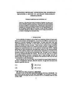
Fig. 1 Interpolation scheme at nodes „a…, and „b… or „c… Fig. 3 Bilinear interpolation

To develop the interpolation scheme for the above boundary condition, we consider a two-dimensional body shown in Fig. 1. In reference to this figure, two different types of nodes are possible, e.g., nodes labeled 共a), or nodes named either 共b兲 or 共c兲, where na, nb, and nc are the unit vectors defining the tangent planes at the corresponding node. Consider first the case of the cell on the left end of Fig. 1 for point labeled 共a兲. This case is shown in Fig. 2共a兲 as point 共p , q兲. In this case, three nodal values 共outside of the body兲 surrounding point 共p , q兲 are known. In the following, for clarity “bars” and

“tildes” are the temperature values inside and outside the body, respectively. ¯ to compute h in Eq. 共10兲, such that Eq. 共11兲 We need to find ⌰ i,j ¯ in the diffusion is satisfied at node 共p , q兲 共the same applies to ⌰ s equation Eq. 共4兲 to find H兲. Thus, we use a bilinear interpolation scheme, as shown in Fig. 3, where ␣ = 关X1 − x1共i,j兲兴 / 关x1共i+1,j兲 ¯ = ⌰共X , X 兲 on −x 兴, ␤ = 共X − x 兲 / 共x −x 兲, and ⌰ 1共i,j兲

2

2共i,j兲

2共i,j+1兲

共p , q兲. This is given as

2共i,j兲

p,q

1

2

¯ = ␣␤⌰ ˜ ˜ ˜ ⌰ p,q i+1,j+1 + ␣共1 − ␤兲⌰i+1,j + 共1 − ␣兲␤⌰i,j+1 ¯ + 共1 − ␣兲共1 − ␤兲⌰ i,j

共12兲

¯ ,⌰ ˜ ¯ On the other hand, the values of auxiliary nodes ⌰ p,j p,j+1, ⌰i,q ˜ and ⌰ , which are required to compute the derivatives for Eq. i+1,q 共11兲, can be obtained by a linear interpolation scheme, with the following expressions: ¯ = ␣⌰ ˜ ¯ ⌰ p,j i+1,j + 共1 − ␣兲⌰i,j

共13a兲

˜ ˜ ¯ ⌰ p,j+1 = ␣⌰i+1,j+1 + 共1 − ␣兲⌰i,j+1

共13b兲

¯ = ␤⌰ ˜ ¯ ⌰ i,q i,j+1 + 共1 − ␤兲⌰i,j

共13c兲

˜ ˜ ˜ ⌰ i+1,q = ␤⌰i+1,j+1 + 共1 − ␤兲⌰i+1,j

共13d兲

On combining Eq. 共11兲 with Eq. 共12兲 and Eqs. 共13a兲–共13d兲, the ¯ can now be written as value for ⌰ i,j

再

¯ = c − ␣␤a⌰ ˜ ⌰ i,j i+1,j+1 −

册

冋

册

冋

␣b ␤b ˜ n2 + ␣共1 − ␤兲a ⌰ n1 i+1,j − ⌬x2 ⌬x1

b ˜ ˜ + 共1 − ␣兲␤a ⌰ n 1⌰ i,j+1 − i+1,q ⌬x1 −

冎冋

共1 − ␣兲b 共1 − ␤兲b b ˜ n 2⌰ n1 + n2 p,j+1 / ⌬x2 ⌬x1 ⌬x2

+ 共1 − ␣兲共1 − ␤兲a

Fig. 2 General interpolation scheme for Dirichlet–Neumann boundary conditions: „a… three nodes outside the boundary; „b… two nodes outside the boundary

1508 / Vol. 129, NOVEMBER 2007

册

共14兲

where n1 and n2 are the projections of n on the x1 and x2 axes, respectively. ⌬x1 and ⌬x2 are the corresponding spatial increments ¯ can be 共see Fig. 2兲. By setting either b = 0 or a = 0 in Eq. 共14兲, ⌰ i,j computed under Dirichlet or Neumann boundary conditions. In the second case, two nodal values surrounding point 共p , q兲 lie inside the body, as shown in Fig. 2共b兲. This case corresponds to the cell on the center of Fig. 1 for point labeled as 共b兲. Apparently, ˜ there are only two known temperatures outside the boundary 共⌰ 3b ˜ 兲 and two unknown temperatures inside the boundary 共⌰ ¯ and ⌰ 4b 1b ¯ 兲. However, we regard ⌰ ¯ as a known quantity, since and ⌰ 2b 2b ¯ =⌰ ¯ , where ⌰ ¯ was previously obtained from Eq. 共14兲 as ⌰ 2b

1a

1a

Transactions of the ASME

Downloaded 21 Nov 2007 to 129.219.244.213. Redistribution subject to ASME license or copyright; see http://www.asme.org/terms/Terms_Use.cfm

Table 1 Comparison in CD, xc, St, and Nu around a cylinder placed in an unbounded flow Re→ Study Kim and Choi 关12兴 Eckert and Soehngen 关29兴 Pan 关30兴 Lima E Silva et al. 关31兴 Current

NuCD

40 xc

Nu

CD

120 St

Nu

CD

150 St

Nu

— — 1.51 1.54 1.53

— — 2.18 — 2.28

3.23 3.48 3.23 — 3.62

— — — — 1.40

— — — — 0.170

5.62 5.69 — — 5.5

— — — 1.37 1.38

— — — 0.170 0.179

— 6.29 — — 6.13

¯ 共=⌰ ¯ of Fig. 1兲 is computed explained above. Therefore, ⌰ i,j 1b with Eq. 共14兲 and the known surrounding values. Equation 共14兲 can be used to determine the temperature values inside the body such that the desired boundary condition is satisfied. The solution procedure involves the following steps. 1. Find a nodal point where we want to satisfy the Robin boundary condition and three nodal points lie outside the body, e.g., node 共a兲 of Fig. 1. 2. Determine temperature ⌰ ¯ 共=⌰ ¯ 兲 from the known suri,j 1a rounding values using Eq. 共14兲. 3. Determine the corresponding node temperature of the adja˜ cent cell, e.g., node 共b兲 of Fig. 1, from Eq. 共14兲 with ⌰ i,j+1 ¯ ¯ ¯ being replaced by ⌰ i,j+1. In this case, ⌰i,j+1 = ⌰1a was previously determined from a bilinear interpolation along with ˜ ,⌰ ˜ ,⌰ ˜ , and the adjacent nodes external to the body ⌰ 2a 3a 4a Eq. 共11兲 being evaluated at node 共a兲, which are all known. 4. Repeat step 3 on the adjacent cell 共right end of Fig. 1兲. 5. Since ⌰ ¯ must equal ⌰ ¯ , this procedure must be repeated 1b 2c until all the nodes near the body have been exhausted, and the difference in values between consecutive iterations is ¯ −⌰ ¯ ⬇ 0. negligible, e.g., ⌰ 1b 2c It is to be noted that the number of iterations required to achieve zero machine accuracy, either for two- or threedimensional simulations, is typically 10 per node.

4

Heat Transfer Simulations

In order to assess the correct implementation of the interpolation algorithm, simulations of four different heat transfer problems are carried out next. 4.1 Forced Convection Over Heated Circular Cylinders. We consider first the forced heat convection over circular cylinders placed in an unbounded uniform flow. Two different cases are analyzed in this section: 共i兲 a single heated cylinder of nondimensional diameter d = 1 and 共ii兲 an arrangement of two heated cylinders, one being the main cylinder of nondimensional diameter d = 1, whereas the other is a secondary cylinder of diameter ds = d / 3. Note that the characteristic length for these problems is Lc = d. For the two cases, the following considerations take place: The fluid is air, and thus Pr= 0.71; the inflow boundary conditions are u1 = 1, u2 = 0, and ⌰ = 0; the outflow boundary conditions are ⳵ui / ⳵t + cu⳵ui / ⳵x1 = 0 and ⳵⌰ / ⳵t + cu⳵⌰ / ⳵x1 = 0 关28兴 共where cu is the space-averaged velocity兲 for i = 1 , 2; the far-field boundary conditions are ⳵ui / ⳵x2 = 0 and ⳵⌰ / ⳵x2 = 0; and the value of the isothermal surface for all the cylinders is ⌰ = 1. The flow is governed by Eqs. 共1兲–共3兲 with P1 = 1 / Re, P2 = Gr/ Re2 共Gr= 0兲, and P3 = 1 / RePr. The computations presented next were carried out using nonuniform grids, which are stretched away from the vicinity of the body using a hyperbolic sine function for test case 共i兲 and a logarithmic function for test case 共ii兲. A number of 1200 grid points inside the cylinder and 112 grid points close to the boundary were used. In all the cases analyzed here, a 400⫻ 400 mesh secured grid independence. During the computations, the Journal of Heat Transfer

time step value was changed dynamically to ensure a CFL= 0.5. In test problem 共i兲, the cylinder was placed at the center of a computational domain of size 30d ⫻ 30d. The center of the cylinder has coordinates 共x1 , x2兲 = 共0 , 0兲, where −15艋 x1 , x2 艋 15. The results shown next were obtained for Re= 兵40, 80, 120, 150其. Table 1 shows a comparison in both the hydrodynamics and the heat transfer of this flow in terms of the drag coefficient CD 1 = FD / 2 ␳U2d, the wake bubble xc or the Strouhal number St = fd / U, and the averaged Nusselt number Nu= ¯hd / k. In the above expressions, FD is the drag force on the cylinder 关13兴, f is the shedding frequency, ¯h is the heat transfer coefficient averaged over its half arc length, and k its thermal conductivity. As can be noted, the present results for both fluid flow and heat transfer compare quantitatively well with the published numerical and laboratory experiments 关12,29–31兴. As an example, for Re= 40, 120, and 150, the differences in Nu against the experiments of Eckert and Soehngen 关29兴 are confined to less than 4%. Figures 4共a兲 and 4共b兲 illustrate the streamlines and temperature contours for Re= 80. From both figures, it can be seen the development of a Kárman vortex street, resembled by the alternating patterns that take place due to vortex shedding, which is typical for this value of Re 关29,32兴. On the other hand, Fig. 5 illustrates a comparison in the local values of the Nu number along the cylinder surface obtained from the proposed scheme and the experiments of Eckert and Soehngen 关29兴 for Re= 120. In the figure, the angle ␸ is measured from the leading edge of the cylinder. As can be noticed, there is a very good agreement between the present results and those of Eckert and Soehngen 关29兴. Also expected is a quantitative increase of the Nu value from 3.62 for Re= 40, to 4.70 for Re= 80, and to 5.50 for Re= 120. The percentage difference between the averaged Nusselt obtained here 共for Re= 120兲 and the experimental one reported by Eckert and Soehngen 关29兴, which is 5.69, is of only 3.4%. Test problem 共ii兲 has been studied experimentally 关32兴 and numerically 关12兴 for different arrangements. Here, we consider two of them for a value of Reynolds number of Re= 80. In the first arrangement, the center of the main cylinder was located at 共x1 , x2兲 = 共−1 , 0兲 with respect to a coordinate system placed at the center of a 30d ⫻ 30d computational domain, whereas the secondary cylinder was centered at 共x1 , x2兲 = 共1 , 1兲. Qualitative results for this problem are depicted in Figs. 6共a兲 and 6共b兲 in terms of the streamlines and isotherms, respectively. In contrast with the forced convection over the single cylinder, shown previously for the same Re number, the figures illustrate how the interaction between the cylinders, for this arrangement, suppresses the vortex shedding and produces a steady flow 关32兴. Qualitatively and quantitatively, these results are in good agreement with the data of Kim and Choi 关12兴. Actual values for the main and secondary cylinders are, respectively, 1.24 and 0.48 for CD, and 4.7 and 3.0 for Nu. Computations were also carried out for an arrangement where the main cylinder was centered at 共x1 , x2兲 = 共−1 , 0兲 and the secondary cylinder at 共x1 , x2兲 = 共1 , 0.5兲. As expected for this arrangement 关12,32兴, our results showed that the flow is unsteady. Again, good agreement with Ref. 关12兴 is found in the values of both CD and Nu NOVEMBER 2007, Vol. 129 / 1509

Downloaded 21 Nov 2007 to 129.219.244.213. Redistribution subject to ASME license or copyright; see http://www.asme.org/terms/Terms_Use.cfm

Fig. 4 Streamlines and temperature contours of flow around cylinder for Re= 80: „a… streamlines; „b… isotherms

for the main and secondary cylinders. Our data for CD are 1.22 and 0.12, and for Nu 4.62 and 1.65, respectively. 4.2 Natural Convection Over a Heated Cylinder Inside a Square Cavity. The proposed algorithm is applied next to simulate the laminar natural convection from a heated cylinder placed eccentrically in a square duct of sides L = 1. The geometry of this validation problem is shown in Fig. 7. The flow and heat transfer are governed by Eqs. 共1兲–共3兲 with P1 = Pr, P2 = RaPr, and P3 = 1, where we have chosen Lc = L as the characteristic length. The cylinder has a nondimensional wall temperature ⌰ = 1, whereas two different sets of thermal boundary conditions are considered for the walls of the cavity: 共i兲 isothermal boundary conditions

Fig. 5 Nu number along cylinder surface for Re= 120. 䊊, present scheme; 〫, experiments by Eckert and Soehngen †29‡.

1510 / Vol. 129, NOVEMBER 2007

where all the walls are maintained at ⌰ = 0, and 共ii兲 isothermal vertical sidewalls at ⌰ = 0 and adiabatic horizontal walls, i.e., ⵜ⌰ · n = 0. For the flow, in both cases, no-slip and no-penetration conditions are applied to all the surfaces. Test case 共i兲 has been studied by Moukalled and Darwish 关33兴 using a bounded skew central-difference scheme, Sadat and Couturier 关34兴 with a meshless diffuse approximation method, and Pan 关30兴 with an unstructured-Cartesian-mesh IB method. The cylinder has a dimensionless diameter d = 0.2, with its center being located at 共x1 , x2兲 = 共−0.15, −0.15兲 as measured from the center of the duct 共see Fig. 7兲. Our calculations were carried out until grid independence was achieved, with grid sizes ranging from 80 ⫻ 80 to 200⫻ 200, for values of the Rayleigh number Ra= 104, 105, and 106. Streamlines and temperature contours for Ra= 104 and Ra= 106 are depicted in Figs. 8 and 9, respectively. As observed, the results shown here agree qualitatively well with those presented in Refs. 关30,33,34兴. Figures 8共a兲 and 8共b兲 illustrate the change on the character of the flow from two well-defined rotating vortices to two distorted ones as Ra is increased from 104 to 106. In the case of the temperature contours, this change is noticed by the shift of the thermal plume now rising toward the left corner of the cavity, as illustrated in Figs. 9共a兲 and 9共b兲. Table 2 shows a quantitative comparison in the values of the average Nusselt Nu number along the cylinder surface for the three values of Ra considered against published data 关30,33,34兴. The maximum difference between the current results and those of Pan 关30兴, for instance, is of only 2%. For test case 共ii兲, in reference to Fig. 7, the cylinder has a dimensionless diameter of d = 0.4, and its center is located at 共x1 , x2兲 = 共0 , 0.1兲 from the center of the duct. This problem has been benchmarked by Demirdžic´ et al. 关35兴. The results obtained from the current algorithm are shown in Figs. 10 and 11. Values of the Nusselt number along the cold walls, obtained with a grid size of 200⫻ 200, are compared in Fig. 10 with those of Demirdžic´ et al. 关35兴, who used half of the domain and a 256⫻ 128 grid. From Transactions of the ASME

Downloaded 21 Nov 2007 to 129.219.244.213. Redistribution subject to ASME license or copyright; see http://www.asme.org/terms/Terms_Use.cfm

Fig. 6 Streamlines and temperature contours of flow around two cylinders for Re= 80: „a… streamlines; „b… isotherms

the figure, it can be seen that the present results overlap with the “exact values” of Demirdžic´ et al. 关35兴. A comparison of the values for the Nusselt number along the cylinder surface, between the present work and that of Demirdžic´ et al. 关35兴, is shown in Fig. 11. In the figure, the azimuthal angle ␸ is measured from top of the cylinder. As before, the agreement of the results obtained from the current scheme as compared to those of Demirdžic´ et al. 关35兴 is excellent. 4.3 Heat Diffusion in an Annulus. We now carry out simulations of the steady and unsteady heat diffusion in an annulus, illustrated schematically in Fig. 12. This problem was studied by

Fig. 7 Cylinder placed eccentrically in a square cavity

Journal of Heat Transfer

Barozzi et al. 关8兴 using an immersed interface 共II兲 method. The diffusion process within the annulus is governed by Eq. 共4兲, with P4 = 1. The annulus is initially at ⌰s,0 = 0, with a uniform temperature ⌰s,e = 0 being applied to the outer surface, and Robin boundary conditions at the internal surface. The present results are compared to the solutions obtained by Barozzi et al. 关8兴 using a nondimensional radius r 苸 关1 , 2兴, where we have used Lc = ri as characteristic length. Three different boundary conditions were applied at the internal boundary in order to test the spatial accuracy of the present formulation. For all cases, the boundary condition at the outer radius is of the Dirichlet type 共⌰s,e = 0兲. The boundary conditions applied at the inner radius were 共a兲 Dirichlet a = 1, b = 0, c = 1; 共b兲 Neumann a = 0, b = 1, c = 1; and 共c兲 mixed a = 1, b = 1, c = 1. Different numbers of regular grid points, ranging from 20⫻ 20 to 120 ⫻ 120 in an uniform Cartesian mesh, were used. For the three boundary conditions above, accuracy of the solutions is presented in terms of the maximum ⑀max- and L2-norm distributions in Figs. 13共a兲–13共c兲, and average values in Table 3. For comparison purposes, the results reported by Barozzi et al. 关8兴 are also included. From the figures, and the table, it can be seen that both techniques achieve second-order accuracy, with actual numerical orders being quantitatively similar. It is to be noted that the uneven distributions of the errors in Figs. 13共b兲 and 13共c兲, as the mesh is refined, may be due to the presence of the irregular boundary whose effect is to produce a local increase in the error when the derivative is computed. The time-dependent system, given in Eq. 共4兲 under general conditions of the inner boundary, is analyzed next, and the results are compared with analytical solutions. Following the procedure described by Carslaw and Jaeger 关36兴, and Özis¸ik 关37兴, the solution of Eq. 共4兲 with ⌰s,0 = 0, ⌰s,e = 0, and a = b = c = 1 in Eq. 共11兲 is given in terms of Bessel series expansions as NOVEMBER 2007, Vol. 129 / 1511

Downloaded 21 Nov 2007 to 129.219.244.213. Redistribution subject to ASME license or copyright; see http://www.asme.org/terms/Terms_Use.cfm

Fig. 8 Streamlines on a 200Ã 200 grid for „a… Ra= 104 and „b… Ra= 106 ⬁

⌰s共r,t兲 =

兺c j=1

j

冋

册

ln共r兲 + 1 J0共␭ jr兲 Y 0共␭ jr兲 exp共− P4␭2j t兲 + − ln共1/2兲 − 1 J0共2␭ j兲 Y 0共2␭ j兲 共15兲

where the eigenvalues, ␭ j for j = 1 , 2 , . . ., are the roots of the equation

cj =

Fig. 9 Isotherms on a 200Ã 200 grid for „a… Ra= 104 and „b… Ra= 106

␭ jJ1共␭ j兲 + J0共␭ j兲 ␭ jY 1共␭ j兲 + Y 0共␭ j兲 − =0 J0共2␭ j兲 Y 0共2␭ j兲 and the constants c j for j = 1 , 2 , . . ., are defined as

共2/␭ j兲兵关J1共␭ j兲/J0共2␭ j兲兴 − 关Y 1共␭ j兲/Y 0共2␭ j兲兴其 4兵关J1共2␭ j兲/J0共2␭ j兲兴 − 关Y 1共2␭ j兲/Y 0共2␭ j兲兴其2 − 关共1/␭2j 兲 + 1兴兵关J0共␭ j兲/J0共2␭ j兲兴 − 关Y 0共␭ j兲/Y 0共2␭ j兲兴其2

In the above equations, J0, Y 0, J1, and Y 1 are the Bessel functions of first and second kinds, of order 0 or 1, respectively. The time-dependent results are shown in Fig. 14 as temperature distributions within the solid annulus at values of the nondimensional time t = 0.15, 0.25, 0.35, and 1.40. From the figure, it can be observed an excellent agreement between the analytical solutions 1512 / Vol. 129, NOVEMBER 2007

共16兲

共17兲

共symbols兲 with those obtained numerically 共solid lines兲. After t = 1.40 nondimensional units, the steady state has been reached, with a value of ⌰s = 0.41 at the inner boundary. The error between the two solutions is confined to less than 1%. The temporal accuracy of the scheme is assessed next by choosing three radii locations within the annulus 共see Fig. 12兲, correTransactions of the ASME

Downloaded 21 Nov 2007 to 129.219.244.213. Redistribution subject to ASME license or copyright; see http://www.asme.org/terms/Terms_Use.cfm

Table 2 Comparison in Nu around a cylinder placed inside a cavity for Ra= 104, 105, and 106 Study Moukalled and Darwish 关33兴 Sadat and Couturier 关34兴 Pan 关30兴 Current

Ra= 104

Ra= 105

Ra= 106

4.741 4.699 4.686 4.750

7.435 7.430 7.454 7.519

12.453 12.421 12.540 12.531

sponding to r = 1.03共PA兲 close to the inner boundary, r = 1.49共PB兲 approximately at the middle plane, and r = 1.94共PC兲 close to the outer boundary. Note that the inner boundary condition is of the Robin type. Different time increments, i.e., ⌬t = 0.2, 0.1, and 0.01, were used, and the results presented in Fig. 13共d兲 in terms of error distributions. From the figure, it is clear that for all the radii locations considered, the scheme is second-order accurate in time. 4.4 Three-Dimensional Forced Convection Over a Heated Sphere. The capacity of the present scheme to handle threedimensional flows is shown next by solving the flow and heat transfer around a heated sphere. Published numerical and experimental results are used to assess the solutions obtained. Thus, let us consider a sphere of nondimensional diameter d = 1, where Lc = d is the characteristic length, placed in an unbounded flow. This flow is governed by Eqs. 共1兲–共3兲 where P1 = 1 / Re, P2 = Gr/ Re2 with Gr= 0, and P3 = 1 / RePr with Pr= 0.71. The boundary conditions for the problem are inflow u1 = 1, u2 = u3 = 0, and ⌰ = 0; outflow ⳵ui / ⳵t + cu⳵ui / ⳵x1 = 0 and ⳵⌰ / ⳵t + cu⳵⌰ / ⳵x1 = 0; and far-field boundaries ⳵ui / ⳵x2 = ⳵ui / ⳵x3 = 0, ⳵⌰ / ⳵x2 = ⳵⌰ / ⳵x3 = 0, respectively, where i = 1 , 2 , 3. The sphere is at a nondimensional temperature ⌰ = 1. The computations were carried out using a 100 ⫻ 100⫻ 100 nonuniform grid, which stretches away from the body to the outer boundaries using a hyperbolic sine function. The sphere is located in the center 共x1 , x2 , x3兲 = 共0 , 0 , 0兲 of a computational cube of size 30d ⫻ 30d ⫻ 30d. The time step value was dynamically changed to ensure a CFL= 0.5. The results from the current approach were obtained for Reynolds numbers Re = 兵50, 100, 150, 200, 220, 300其. Figures 15共a兲–15共e兲 illustrate the streamlines and isotherms on the symmetry plane x3 = 0 for Re= 50, 100, 150, 200, and 220, respectively. The streamlines presented in Figs. 15共a兲–15共d兲 show that the flow is steady and separated, with an axisymmetric recirculation bubble that grows as the Reynolds number increases.

Fig. 10 Nu number along cold wall for Ra= 106 and Pr= 10. 〫, present scheme; 䊊, Demirdžic´ et al. †35‡.

Journal of Heat Transfer

Fig. 11 Nu number along cylinder surface for Ra= 106 and Pr = 10. Angle ␸ is measured from top of cylinder. 〫, present scheme; 䊊, Demirdžic´ et al. †35‡.

Quantitatively, the present results for both drag coefficient CD and wake bubble xc are in good agreement with those of Marella et al. 关4兴 and Johnson and Patel 关38兴. Actual values for Re= 50, 100, and 150 are 1.62, 1.07, and 0.85 for CD, and 0.42, 0.90, and 1.23 for xc, respectively. For Re= 220, Fig. 15共e兲 shows the expected axial asymmetry of the flow, which has been experimentally determined to occur in the Re苸 关210, 270兴 range 关39兴. The corresponding isotherms, shown also in Figs. 15共a兲–15共e兲, reflect the behavior of the flow. As the Reynolds number increases, the isotherms in the wake of the sphere become more distorted due to the amount of recirculating flow. Though small values of the heat transfer coefficient are characteristics of this region, it can be seen that in the rear of the sphere 共at an angle of approximately 180 deg兲, the heat transfer coefficient is increased locally with Re number. The computed values of the Nusselt number averaged over the surface of the sphere Nu are 4.99, 7.00, 8.27, 9.19, and 9.30 for Re= 50, 100, 150, 200, and 220, respectively. These results are in good agreement with the correlation developed by Feng and Michaelides 关40兴, for the same conditions. The maximum difference between the corresponding values is less

Fig. 12 Concentric cylindrical annulus

NOVEMBER 2007, Vol. 129 / 1513

Downloaded 21 Nov 2007 to 129.219.244.213. Redistribution subject to ASME license or copyright; see http://www.asme.org/terms/Terms_Use.cfm

Fig. 13 „„a…–„c…… L2 norm and maximum norm „⑀max… as functions of the mesh size ␦ for different inner boundary conditions. „d… Error versus ⌬t for inner Robin boundary conditions. „a… Dirichlet „a = 1, b = 0, c = 1…. „b… Neumann „a = 0, b = 1, c = 1…. „c… Robin „a = 1, b = 1, c = 1…. „d… Radii locations: 〫, PA; 䊊, PB; 䉭, PC.

than 8%. Increasing the Reynolds number beyond 270 eventually leads to unsteady flow 关38兴. For Re= 300, Fig. 16 illustrates the vortical structures of the flow obtained with the method proposed by Hunt et al. 关41兴 共more in-depth details are in Refs. 关42,43兴兲. As seen in the figure, these vortical structures resemble very well the established vortex shedding. The average values of the drag coefficient CD = 0.570 and the Strouhal number St= 0.133 compare well to those of Marella et al. 关4兴 and Johnson and Patel 关38兴. For this value of Re number, the averaged Nusselt number Nu= 10.50 deviates from that given by Feng and Michaelides 关40兴 correlation in only 3.6%.

5

boundary conditions within the context of the IB methodology. An advantage of this algorithm is that both Dirichlet and Neumann conditions can be naturally implemented by setting appropriate values to the constants in the most general linear equation. Its

Concluding Remarks

In the current work, we have presented a novel interpolation scheme that is able to handle either Dirichlet, Neumann, or mixed Table 3 Numerical order of accuracy in terms of ⑀max and L2 for the annulus problem Dirichlet

Neumann

Robin

Method / BC →

L2

⑀max

L2

⑀max

L2

⑀max

Barozzi et al. 关8兴 Current

1.91 2.16

1.93 2.09

2.05 2.02

1.99 1.93

2.02 2.03

1.95 1.93

1514 / Vol. 129, NOVEMBER 2007

Fig. 14 Numerical „solid lines… versus analytical „symbols… time-dependent solutions. -䉭-, t = 0.15; -〫-, t = 0.25; -䊊-, t = 0.35; -䉮-, t = 1.40 „steady state….

Transactions of the ASME

Downloaded 21 Nov 2007 to 129.219.244.213. Redistribution subject to ASME license or copyright; see http://www.asme.org/terms/Terms_Use.cfm

Fig. 16 Oblique view of vortical structures of flow for Re = 300

validation has been assessed by favorable comparison with numerical results available in the literature and/or analytical solutions for different heat transfer problems: forced heat convection over circular cylinders, natural heat convection over a cylinder placed inside a cavity, steady and unsteady diffusion of heat inside an annulus, and three-dimensional forced convection over a sphere. The interpolation algorithm developed here provides a method that is second-order accurate in space and time and is suitable for analyzing heat transfer phenomena in single or multiple bodies with complex boundaries on two- and threedimensional Cartesian meshes.

Acknowledgment The authors thank Professor R.L. Street of Stanford University for providing the multigrid subroutine used in this work and to G. Constantinescu of University of Iowa for his assistance with the vortex visualization. A. P.-V. also acknowledges financial support from PROMEP, México through grants PROMEP/PTC-68 and PROMEP-CA9/FCQ-UASLP, and FAI/UASLP research fund. We are grateful for the helpful comments of the anonymous referees which improved the quality of the manuscript. Computational resources for this work were provided by the Ira A. Fulton High Performance Computing Initiative at ASU.

Nomenclature a,b,c cj cu e f h,H Lc L2 n1 , n2 P1 , P2 , P3 , P4 PA , PB , PC r u xc xi x1共i,j兲 , x2共i,j兲

⫽ ⫽ ⫽ ⫽ ⫽ ⫽ ⫽ ⫽ ⫽ ⫽ ⫽ ⫽ ⫽ ⫽ ⫽ ⫽

constants in general boundary condition jth constant in Eq. 共15兲 space-averaged velocity unit vector in vertical direction momentum forcing energy forcing characteristic length Euclidean norm projections on x1 and x2 axes of unit vector n nondimensional parameters radii locations radius Cartesian velocity vector wake bubble Cartesian coordinates coordinates based on node 共i , j兲 for bilinear interpolation X1 , X2 ⫽ coordinates of immersed-boundary node

Fig. 15 Streamlines and temperature contours for flow around a sphere in the 50Ï ReÏ 220 range. „a… Re= 50, „b… Re= 100, „c… Re= 150, „d… Re= 200, and „e… Re= 220.

Journal of Heat Transfer

Greek Symbols ␣ ⫽ thermal diffusivity of fluid, interpolation factor ␣s ⫽ thermal diffusivity of solid ␤ ⫽ coefficient of thermal expansion, interpolation factor ⌬x1 , ⌬x2 ⫽ spatial increments in x1 and x2 directions ␦ ⫽ mesh size ⑀ ⫽ error ⑀max ⫽ maximum norm ␭ j ⫽ jth eigenvalue ⵜ ⫽ Nabla operator ⌰ ⫽ normalized temperature ⌰s ⫽ normalized temperature within the solid ⌰s,0 ⫽ normalized initial temperature within the solid NOVEMBER 2007, Vol. 129 / 1515

Downloaded 21 Nov 2007 to 129.219.244.213. Redistribution subject to ASME license or copyright; see http://www.asme.org/terms/Terms_Use.cfm

⌰⬁ ⫽ normalized reference fluid temperature ¯ ⫽ temperature on or inside the body ⌰ ˜ ⫽ temperature outside the body in energy-forcing ⌰ interpolation ␸ ⫽ reference angle Subscripts and Superscripts e ⫽ outer-boundary value i , j ⫽ indices for the Cartesian coordinates n ⫽ index for time step

References 关1兴 Peskin, C. S., 1972, “Flow Patterns Around Heart Valves: A Numerical Method,” J. Comput. Phys., 10, pp. 252–271. 关2兴 Peskin, C. S., 2002, “The Immersed Boundary Method,” Acta Numerica, 11, pp. 479–517. 关3兴 Udaykumar, H. S., Mittal, R., and Rampunggoon, P., 2002, “Interface Tracking Finite Volume Method for Complex Solid-Fluid Interactions on Fixed Meshes,” Commun. Numer. Methods Eng., 18, pp. 89–97. 关4兴 Marella, S., Krishnan, S., Liu, H., and Udaykumar, H. S., 2005, “Sharp Interface Cartesian Grid Method I: An Easily Implemented Technique for 3D Moving Boundary Computations,” J. Comput. Phys., 210, pp. 1–31. 关5兴 Liu, H., Krishnan, S., Marella, S., and Udaykumar, H. S., 2005, “Sharp Interface Cartesian Grid Method II: A Technique for Simulating Droplet Impact on Surfaces of Arbitrary Shape,” J. Comput. Phys., 210, pp. 32–54. 关6兴 Yang, Y., and Udaykumar, H. S., 2005, “Sharp Interface Cartesian Grid Method III: Solidification of Pure Materials and Binary Solutions,” J. Comput. Phys., 210, pp. 55–74. 关7兴 Lee, L., Li, Z., and LeVeque, R. J., 2003, “An Immersed Interface Method for Incompressible Navier-Stokes Equations,” SIAM J. Sci. Comput. 共USA兲, 25共3兲, pp. 832–856. 关8兴 Barozzi, G. S., Bussi, C., and Corticelli, M. A., 2004, “A Fast Cartesian Scheme for Unsteady Heat Diffusion on Irregular Domains,” Numer. Heat Transfer, Part B, 46共1兲, pp. 59–77. 关9兴 Fogelson, A. L., and Keener, J. P., 2001, “Immersed Interface Methods For Neumann and Related Problems in Two and Three Dimensions,” SIAM J. Sci. Comput. 共USA兲, 22共5兲, pp. 1630–1654. 关10兴 Kim, J., Kim, D., and Choi, H., 2001, “An Immersed-Boundary Finite-Volume Method For Simulations Of Flow In Complex Geometries,” J. Comput. Phys., 171, pp. 132–150. 关11兴 Zhang, L., Gerstenberger, A., Wang, X., and Liu, W. K., 2004, “Immersed Finite Element Method,” Comput. Methods Appl. Mech. Eng., 193, pp. 2051– 2067. 关12兴 Kim, J., and Choi, H., 2004, “An Immersed-Boundary Finite-Volume Method for Simulations of Heat Transfer in Complex Geometries,” KSME Int. J., 18共6兲, pp. 1026–1035. 关13兴 Pacheco, J. R., Pacheco-Vega, A., Rodic´, T., and Peck, R. E., 2005, “Numerical Simulations of Heat Transfer and Fluid Flow Problems Using an Immersed-Boundary Finite-Volume Method on Nonstaggered Grids,” Numer. Heat Transfer, Part B, 48, pp. 1–24. 关14兴 Fadlun, E. A., Verzicco, R., Orlandi, P., and Mohd-Yusof, J., 2000, “Combined Immersed-Boundary Finite-Difference Methods for Three-Dimensional Complex Flow Simulations,” J. Comput. Phys., 161, pp. 35–60. 关15兴 Mittal, R., and Iaccarino, G., 2005, “Immersed Boundary Methods,” Annu. Rev. Fluid Mech., 37, pp. 239–261. 关16兴 Tyagi, M., and Acharya, S., 2005, “Large Eddy Simulation of Turbulent Flows in Complex and Moving Rigid Geometries Using the Immersed Boundary Method,” Int. J. Numer. Methods Fluids, 48, pp. 691–722. 关17兴 Deuflhard, P., and Hochmuth, R., 2004, “Multiscale Analysis of Thermoregulation in the Human Microvascular System,” Math. Methods Appl. Sci., 27, pp. 971–989. 关18兴 Oyanader, M. A., Arce, P., and Dzurik, A., 2003, “Avoiding Pitfalls in Electrokinetic Remediation: Robust Design and Operation Criteria Based on First Principles For Maximizing Performance in a Rectangular Geometry,” Electrophoresis, 24共19–20兲, pp. 3457–3466.

1516 / Vol. 129, NOVEMBER 2007

关19兴 DeLima-Silva, W., Jr., and Wrobel, L. C., 1995, “A Front-Tracking BEM Formulation for One-Phase Solidification/Melting Problems,” Eng. Anal. Boundary Elem., 16, pp. 171–182. 关20兴 Amaziane, B., and Pankratov, L., 2006, “Homogenization Of A ReactionDiffusion Equation With Robin Interface Conditions,” Appl. Math. Lett., 19共11兲, pp. 1175–1179. 关21兴 Sparrow, E. M., and Gregg, J. L., 1958, “Similar Solutions for Free Convection From a Non-Isothermal Vertical Plate,” ASME J. Heat Transfer, 80, pp. 379–386. 关22兴 Leonard, B. P., 1979, “A Stable And Accurate Convective Modelling Procedure Based on Quadratic Upstream Interpolation,” Comput. Methods Appl. Mech. Eng., 19, pp. 59–98. 关23兴 Zang, Y., Street, R. L., and Koseff, J. F., 1994, “A Non-Staggered Grid, Fractional Step Method for Time Dependent Incompressible Navier-Stokes Equations in Curvilinear Coordinates,” J. Comput. Phys., 114, pp. 18–33. 关24兴 Pacheco, J. R., 1999, “On the Numerical Solution of Film and Jet Flows,” Ph.D thesis, Department Mechanical and Aerospace Engineering, Arizona State University, Tempe. 关25兴 Pacheco, J. R., and Peck, R. E., 2000, “Non-Staggered Grid Boundary-Fitted Coordinate Method for Free Surface Flows,” Numer. Heat Transfer, Part B, 37, pp. 267–291. 关26兴 Pacheco, J. R., 2001, “The Solution of Viscous Incompressible Jet Flows Using Non-Staggered Boundary Fitted Coordinate Methods,” Int. J. Numer. Methods Fluids, 35, pp. 71–91. 关27兴 Mohd-Yusof, J., 1997, “Combined Immersed-Boundary/B-Spline Methods For Simulations of Flows in Complex Geometries,” CTR Annual Research Briefs, NASA Ames/Stanford University, Stanford, CA, pp. 317–327. 关28兴 Orlanski, I., 1976, “A Simple Boundary Condition For Unbounded Hyperbolic Flows,” J. Comput. Phys., 21, pp. 251–269. 关29兴 Eckert, E. R. G., and Soehngen, E., 1952, “Distribution of Heat-Transfer Coefficients Around Circular Cylinders in Crossflow At Reynolds Numbers From 20 to 500,” Trans. ASME, 75, pp. 343–347. 关30兴 Pan, D., 2006, “An Immersed Boundary Method on Unstructured Cartesian Meshes for Incompressible Flows With Heat Transfer,” Numer. Heat Transfer, Part B, 49, pp. 277–297. 关31兴 Lima E Silva, A. L. F., Silveira-Neto, A., and Damasceno, J. J. R., 2003, “Numerical Simulation of Two-Dimensional Flows over a Circular Cylinder Using the Immersed Boundary Method,” J. Comput. Phys., 189, pp. 351–370. 关32兴 Strykowski, P. J., and Sreenivasan, K. R., 1990, “On the Formation and Suppression of Vortex Shedding at Low Reynolds Numbers,” J. Fluid Mech., 218, pp. 71–107. 关33兴 Moukalled, F., and Darwish, M., 1997, “New Bounded Skew Central Difference Scheme, Part II: Application to Natural Convection in an Eccentric Annulus,” Numer. Heat Transfer, Part B, 31, pp. 111–133. 关34兴 Sadat, H., and Couturier, S., 2000, “Performance and Accuracy of a Meshless Method for Laminar Natural Convection,” Numer. Heat Transfer, Part B, 37, pp. 455–467. 关35兴 Demirdžic´, I., Lilek, Ž., and Peric´, M., 1992, “Fluid Flow and Heat Transfer Test Problems for Nonorthogonal Grids: Bench-Mark Solutions,” Int. J. Numer. Methods Fluids, 15, pp. 329–354. 关36兴 Carslaw, H. S., and Jaeger, J. C., 1986, Conduction of Heat in Solids, 2nd ed., Oxford University Press, Oxford. 关37兴 Özisik, M. N., 1989, Boundary Value Problems of Heat Conduction, Dover, Mineola, NY. 关38兴 Johnson, T. A., and Patel, V. C., 1999, “Flow Past a Sphere up to Reynolds Number of 300,” J. Fluid Mech., 378, pp. 19–70. 关39兴 Magarvey, R. H., and Bishop, R. L., 1961, “Transition Ranges for ThreeDimensional Wakes,” Can. J. Phys., 39, pp. 1418–1422. 关40兴 Feng, Z.-G., and Michaelides, E. E., 2000, “A Numerical Study on the Transient Heat Transfer From a Sphere at High Reynolds and Peclet Numbers,” Int. J. Heat Mass Transfer, 43, pp. 219–229. 关41兴 Hunt, J. C. R., Wray, A. A., and Moin, P., 1988, “Eddies, Stream, and Convergence Zones in Turbulent Flows,” Proceedings of the 1988 CTR Summer Program, NASA Ames/Stanford University, Stanford, CA, pp. 193–208. 关42兴 Constantinescu, S. G., and Squires, K. D., 2004, “Numerical Investigation of the Flow Over a Sphere in the Subcritical and Supercritical Regimes,” Phys. Fluids, 16共5兲, pp. 1449–1467. 关43兴 Jeong, J., and Hussain, F., 1995, “On the Identification of a Vortex,” J. Fluid Mech., 285, pp. 69–94.

Transactions of the ASME

Downloaded 21 Nov 2007 to 129.219.244.213. Redistribution subject to ASME license or copyright; see http://www.asme.org/terms/Terms_Use.cfm