Radiation boundary conditions for the numerical ... - CiteSeerX

www.DownloadPaper.ir Ada Numerica (1999), pp. 47-106

© Cambridge University Press, 1999

Radiation boundary conditions for the numerical simulation of waves Thomas Hagstrom* Department of Mathematics and Statistics, The University of New Mexico. Albuquerque, NM 87131, USA E-mail: hagstromSmath.unm.edu

We consider the efficient evaluation of accurate radiation boundary conditions for time domain simulations of wave propagation on unbounded spatial domains. This issue has long been a primary stumbling block for the reliable solution of this important class of problems. In recent years, a number of new approaches have been introduced which have radically changed the situation. These include methods for the fast evaluation of the exact nonlocal operators in special geometries, novel sponge layers with reflectionless interfaces, and improved techniques for applying sequences of approximate conditions to higher order. For the primary isotropic, constant coefficient equations of wave theory, these new developments provide an essentially complete solution of the numerical radiation condition problem. In this paper the theory of exact boundary conditions for constant coefficient time-dependent problems is developed in detail, with many examples from physical applications. The theory is used to motivate various approximations and to establish error estimates. Complexity estimates are also derived to compare different accurate treatments, and an illustrative numerical example is given. We close with a discussion of some important problems that remain open.

Supported, in part, by NSF Grant DMS-9600146, the Institute for Computational Mechanics in Propulsion (ICOMP), NASA, Lewis Research Center, Cleveland, Ohio; DARPA/AFOSR Contract F49620-95-C-0075; and, while in residence at the Courant Institute. DOE Contract DEFGO288ER25053.

www.DownloadPaper.ir 48

T. HAGSTROM

CONTENTS 1 Introduction 2 Formulations of exact boundary conditions 3 Approximations and implementations 4 Conclusions and open problems References

48 50 76 100 103

1. Introduction Problems in wave propagation have played and will continue to play a central role in the mathematical analysis of physical and biological systems. A defining feature of most wave problems is the radiation of energy to the far field. Mathematically, this is naturally modelled by the use of an unbounded domain, with the addition, in frequency domain problems, of a radiation boundary condition at infinity. In numerical simulations, the accurate approximation of radiation to the far field is also crucial. As it is impossible to solve directly a problem posed on an unbounded domain, new techniques, such as the introduction of an artificial boundary and associated radiation boundary conditions, are needed. The goal of this article is to outline the development, implementation, and analysis of various practical methods for solving this problem for some important models, and to present what I believe is a useful mathematical framework in which to pursue improvements and extensions. Although wave propagation is inherently a time-dependent phenomenon, it has been fruitful in many settings to solve linear problems in the frequency domain. Approaches to the accurate solution of elliptic boundary value problems on unbounded domains are, generally, far better developed than their time domain analogues. Useful techniques include a variety of boundary integral methods, which may be applied on physical or artificial boundaries, including classical integral equations of potential theory (Greengard and Rokhlin 1997, Rokhlin 1990), extensions of Calderon-Seeley equations (Ryabenkii 1985), the Dirichlet-to-Neumann map (Givoli 1992) and infinite elements (Bettess 1992, Demkowicz and Gerdes 1999). Moreover, the efficiency of solving the classical equations has been greatly enhanced in the past decade through the introduction of the fast multipole method. The aims of the numerical analysis of partial differential equations on unbounded domains are clear. We seek methods which: (i) can automatically achieve any prescribed accuracy on bounded subsets of the original domain, (ii) in terms of both computation and storage, cost no more than the solution of a standard problem on the bounded subdomain.

www.DownloadPaper.ir RADIATION BOUNDARY CONDITIONS

49

Though certainly more research and development is called for, it is my opinion that these goals have been or can be met by the methods mentioned above for most elliptic problems. An exception to this is the difficult case of Helmholtz-type equations with general variable coefficients at infinity. The situation with time-dependent problems has been far less satisfactory. The general belief was that exact domain reductions, which necessarily involve history-dependent operators, could never be made computationally feasible. As a result, various simple approximations were employed. These easily met the second criterion, but their accuracy was often poorly understood. Although the approximate conditions proposed were typically embedded in a hierarchy of conditions of increasing order and, presumably, accuracy, as in Lindman (1975), Engquist and Majda (1977, 1979), and Bayliss and Turkel (1980), the hierarchy was rarely used. For some problems it seemed that good results were obtained with the low-order approximations. However, there was generally no way to monitor or decrease the error automatically. Moreover, as we shall see later, it is possible to pose very simple problems for which the standard methods produce inaccurate results. Clearly, our first criterion is not met by the simpler techniques, which from the point of view of the numerical analyst is completely unacceptable. In the past few years, the situation has radically changed, at least for the basic, constant coefficient equations of wave theory. Progress has been made on many fronts, including: (i) the development of efficient algorithms for evaluating exact, temporally nonlocal boundary operators through the use of exact or uniformly accurate rational representations of the transforms of their associated convolution kernels, (ii) the development of improved sponge layer techniques exhibiting reflectionless interfaces with the lossless interior domains, (iii) improved techniques for the implementation to higher orders of the older hierarchies of approximate conditions, along with improvements in the analysis of their convergence with increasing order. In this article, I hope to give a broad exposition from a unified viewpoint of the developments listed above. The reader should be cautioned from the outset that, in comparison with typical theories in computational mathematics, what follows may seem rather specialized. We deal with special equations, often restrict ourselves to special boundaries, and make use of special functions. That said, the results themselves have enormous applicability as the equations we can successfully treat include many of the most important in applications. Moreover, it is not unreasonable to hope that some of these methods will be generalizable to problems we cannot now solve.


T. HAGSTROM

Our approach to the theory of radiation boundary conditions is straightforward. First, we construct exact boundary conditions. Although such conditions can be described in some generality as certain projections of boundary data, we concentrate on concrete expressions derived by separation of variables. For artificial boundaries that satisfy a scale invariance condition, the exact condition factors into the composition of nonlocal spatial and temporal operators. Approximate conditions are analysed using the standard concepts: stability and consistency. From this analysis we obtain sharp error estimates for a wide variety of techniques. These error bounds are used to estimate the computational complexity of the competing methods. The results are also illustrated by a simple numerical experiment. It should be noted that a comprehensive body of numerical results on an appropriate set of benchmark problems is lacking. There has been interest in developing such a set (see Geers (1998)), and I am of the opinion that the problems used here and in Alpert, Greengard and Hagstrom (1999 a) and Hagstrom and Goodrich (1998) are particularly useful, due both to the simplicity of their definition and to the difficulty of their solution. What I have not tried to do is give a comprehensive survey of the many contributions to this subject that have appeared over the past twenty years. The reader is referred to the survey articles (Givoli 1991, Tsynkov 1998) which have extensive bibliographies. I do make many references to the literature within the text, but these are primarily intended to aid the reader who wishes to delve into the subject more deeply, rather than to provide an accurate historical record of its development. Finally I would like to acknowledge the important contributions of those who collaborated with me on a variety of research projects in this field: Brad Alpert, John Goodrich, Leslie Greengard, S. I. Hariharan, H. B. Keller, Jens Lorenz, Richard MacCamy, Jan Nordstrom, and Liyang Xu. I also acknowledge the support of the NSF, the Institute for Computational Mechanics in Propulsion (NASA), DARPA/AFOSR, and, for work done while in residence at the Courant Institute, DOE. Throughout I have tried to emphasize the personal nature of the conclusions expressed herein through the use of the first person, and take full responsibility for them. 2. Formulations of exact boundary conditions In this section I briefly develop the theory of exact boundary conditions for time-dependent problems and apply it to derive explicit expressions for a long list of problems with simple artificial boundaries. The list includes the scalar wave equation and its dispersive analogue, Maxwell's equations, the linear elasticity equations, the advection-diffusion equation, the Schrodinger equation, the linearized compressible Euler equations, and the linearized incompressible Navier-Stokes equations. My purpose in presenting so many


51

examples, aside from the inherent physical interest in all of them, is to demonstrate the remarkable unity of the problem. In particular, although the details of each calculation differ, the recipe for carrying them out does not. Moreover, we shall see that the same few convolution kernels reappear in example after example to define the temporally nonlocal part of the exact condition. Practically, this means that the accurate approximation or compression of a rather small number of operators will have extensive applications. I will show how this can be done in the second part of this article. The outline of the theory of exact conditions presented here has been known for some time (Gustafsson and Kreiss 1979, Hagstrom 1983). However, it was only recently used to develop and analyse efficiently implementable but arbitrarily accurate approximations. The equations considered fall into two classes: hyperbolic equations for which the spatial and temporal operators have the same order, and equations which are first order in time but second order in space. Viewed as pseudodifferential operators, the exact conditions in each case are of different types. As a result our techniques for separating them into local and nonlocal parts differ.

2.1. The scalar wave equation The scalar wave equation is the most ubiquitous model of wave propagation and, hence, is the natural starting point for our study. Consequently, the vast majority of work on the subject has been devoted to this case. I will proceed from the general to the particular, ending with useful expressions for exact conditions on planar, spherical and cylindrical artificial boundaries. General boundaries We consider a mixed problem for the inhomogeneous wave equation in an unbounded domain, Q: 2 C

V 2 « + / , t > 0 , xefl,

(2.1)

with initial and boundary conditions: u(x, 0) = uo(x), a

du — (:z, 0) = vo(x),

(2.2)

7T+0l£+'yu = 9, zecKl (2.3) On dt To truncate the problem, we choose a bounded subdomain, T c f i , which we assume contains the support of the data, / , uo, Vo and g. The boundary of T then consists of two parts, £ C dfl and what we will call the artificial boundary, T. For example, if we are solving an exterior problem, that is, if


T. HAGSTROM

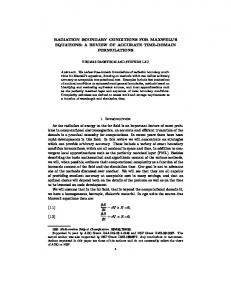
Fig. 1. Domains for an exterior problem: E is the tail, T is the computational domain, T is the artificial boundary

the domain ft is the complement of some finite number of finite domains, then X will consist of the boundaries of these regions while F will be some closed surface which surrounds them. (See Figure 1.) In T we solve (2.1), (2.2) and (2.3) supplemented by an additional boundary condition on F: (2.4) Beu = 0, x We term the boundary condition (2.4) exact if the truncated problem has a unique solution which, for all t > 0, coincides with the restriction to T of the solution of the original problem posed on the unbounded domain Q. Note that we insist on a homogeneous boundary condition on F, so that it will be explicitly independent of the data. If we allowed the support of these to extend beyond T an inhomogeneous condition would generally be required. An indirect description of Be may be derived as follows. Consider the part of the domain 'discarded' as we pass from Q to T, i.e., the 'tail', E = f2 — T. Consider the set, S, consisting of all solutions of the homogeneous wave equation in H, with zero initial data and satisfying the boundary condition (2.3) with g = 0 on that part of dE which is also part of d£l. As we have as yet imposed no boundary condition on F, we expect that S will be infinite.


53

Now the restriction to S from Q. of the solution, u, to our original problem must be an element of S. Moreover, so long as the trace on F of a solution of (2.1), (2.2), (2.3) in T, along with the trace of its normal derivative, coincide with the traces of an element, w, of ?7>0. We have also introduced

(2.6)

(2.7)

s

s = -. c

At least for r\ sufficiently large, we also require that u be bounded and assume that a, /?, 7 are real and a,(3>0. For our purposes, it is simplest to parametrize the transforms of elements of S by their boundary values at F. In particular, given some sufficiently smooth function w(x, s) defined on F, there exists a unique solution, u, of (2.5)-(2.6) such that u(x, s) = w(x, s), x G F. See, for instance, Ramm (1986) for proofs in various unbounded domains. Now we may compute the trace of the normal derivative (outward for T) of


T. HAGSTROM

this solution on F, which defines the so-called Dirichlet-to-Neumann map,

-t>:

du

Vw, x e r.

an Denoting Laplace transformation by C, our exact boundary operator Be may thus be denned by Beu = ~ + ZT 1 (l>£u) . (2.8) on ^ s We note that Be is not a local {i.e., differential) operator. This fact has led to the conclusion that direct implementations of the exact condition are uneconomical: a conclusion we shall demonstrate to be false for some special choices of the artificial boundary. One way to express V is in terms of the Green's function for the problem in H. Let G(x, y, s) satisfy

along with (2.6) (in y) and G = 0,

Then, for x g F , A

/ N

d

[ dG dG,

, , , ,

-Vw(x) = - - — / -—{x,y,s)w{y)dy. onx Jr ony (This equation must be interpreted in terms of limits as x —> F.) For purposes of computation, it is most convenient to express V in terms of its eigenvalues and eigenfunctions, that is, oo

Vw(y,s) = ^\j{s)Yj(y,s)

.

/ Y*(z,s)w(z,s)dz.

In special cases this representation further simplifies, as the eigenfunctions, Yj, turn out to be independent of s. Then the nonlocality may be expressed as the composition of a spatial and temporal operator, each of which may be amenable to a 'fast' evaluation. The invariance of the eigenfunctions with s follows from a scale invariance of the artificial boundary. Boundaries for which it holds include planes, spheres, cylinders and cones. Detailed expressions for Be in these cases are developed below. We finally note that extensions of the solution in S from F to another boundary F' C H may be used in lieu of the exact boundary condition. Precisely, it follows from causality that for any x' € F ' we may derive rep-


55

resentations of the form

u(x',t') = f

[ [KD(x',x,t',t)u{x,t)+

Jt

= 0.

(2.18,

The rationality of 5) implies that the temporal convolution in (2.18) can be localized, that is. its equivalent to the solution of a differential equation, albeit of order I. T h e localizability of the exact boundary condition was first noted and used by Sofronov (1993) and Grote and Keller (1995, 1996). We also have the following beautiful continued fraction representation for Si, which will play a role in efficient implementations of the exact condition: o ^

_

M (

~

}

-

W + D 9

1 | i

,

1

2

+ 2

4

l-+

Z

x

r 9 l q

m+i)—2—• 4 ( - + ' ( ' + >- ' +

4(

2

2

( 3 N

1

9

)

l

+ 3+..0 J

It is also possible to derive analogous expressions for sphcre-to-sphere ex tension operators. As mentioned earlier, these can be used in lieu of bound ary conditions. The properties of localizability and ease of approximation which (2.18) possesses remain valid for the extension operators. In fact it is the extension formulation that is implemented in Sofronov (1999). The construction of exact conditions on a spherical boundary is directly generalizable to conical domains. Precisely, we suppose E may be described in spherical coordinates by E = { ( p . M ) e (R.oc)

x0},

and that appropriate boundary conditions are imposed on 9 0 . Then we may separate variables as before except that we must expand in terms of the eigenfunctions of the Beltrami operator on 0 and. in (2.14), we must replace —1(1 + 1) by the eigenvalues —Kf- Then the transform of the exact boundary condition is as in (2.16) except that the index of the modified Bessel functions is

Of course, for these indices, the exact condition is no longer a rational func tion of s, so that the operators are not equivalent to local operators in time. However, as we shall see later, this does not preclude their effective implementation. Cylindrical

boundary

We now take T to be the infinite cylinder described in standard cylindrical coordinates, (r.6,z), by r — R. Note that, just as in the case of a planar boundary, we may restrict z to a finite interval with the addition of appro priate boundary conditions and may also replace d /dz by a more general 2

2


59

Sturm-Liouville operator. In the formulas that follow, this would simply require replacing Fourier transforms in z by Fourier series. Thus, with k denoting the Fourier dual variable to z and I indexing the Fourier series in 9, we derive the ordinary differential equation =0

(2.20)

r Or in the tail, with bounded solutions for Re s > 0 given by

ui = Ai(s, k)Ki(r\/s2 + k2). Here, again, K\ denotes the modified Bessel function of the third kind (Abramowitz and Stegun 1972, Ch. 9). Using the well-known asymptotic expansions of K\ for large argument, found, for example, in the previously noted reference,

we may again express the temporal part of the boundary condition as the sum of a local operator and convolution with a function. Precisely: V,

= s + —- + (Vs2 + k2-s) + -,Cl(RVs2 + k2),

In the time domain we have

Tu = (ck2K(c\k\t) * u + —^(Gtict,R,

k) * (Fou))\ ,

where Te,z represents Fourier transformation in 6 and z, respectively, and

This result can be extended to domains where 9 is restricted to a subinterval of (#0J#I) £ (0, 2TT) and additional boundary conditions are imposed. Then we need only change the index of the Bessel functions in (2.21) from I to KI where — nf is the Ith. eigenvalue of d2/d92. We note that, in contrast with the spherical case, condition (2.22) cannot be exactly localized in time. However, as previously mentioned, the operators in all three cases may be very accurately and efficiently approximated


T. HAGSTROM

using essentially the same techniques. In particular, it is possible to express Ci as the sum of a rational function and a function denned as an integral. Convergent approximations are derived in Sofronov (1999) by discretizing the integral. Similarly, the transform of the planar kernel may be expressed in integral form, and convergent approximations are derived in Hagstrom (1996) by discretization. In subsequent sections we will outline how these representations can be combined with multipole expansions to develop uniform approximations as in Alpert, Greengard and Hagstrom (19996). The dispersive wave equation The dispersive wave equation is given by ^

VW

(2.23)

Exact boundary conditions for (2.23) have precisely the same form as those for the wave equation, except that eigenvalues used in the definition of the nonlocal operators are shifted by one. Therefore we have, on a planar boundary, from (2.12):

On a sphere, using (2.18), we have

0+

!

^

where ~

/{(Rs)~1/2Kl/(Rs))'

l\

and

Note that this condition is not temporally localizable. Finally, on a cylindrical boundary, we adapt (2.22):

tu = (crfKicryt) * u + ê\Gi{ct, where 7 = yj\k\2 + l, and Ci is given by (2.21).

Gi

R, k) *


61

2.2. Generalizations to hyperbolic systems Consider now a general first-order hyperbolic system with artificial boundary F given by the hyperplane x = 0, denoting as above the tangential variables by y. The equation in the tail takes the form du

v-^ _, du

,n

,.

where u € M9, AQ,BJ € Rqxq. We assume strong hyperbolicity. (See Kreiss and Lorenz (1989).) This implies, among other things, that the eigenvalues of P = ii k0A0

V

are purely imaginary for real kj. To simplify the algebra, we also assume that the artificial boundary is noncharacteristic: that is, AQ is invertible. Solving for du/dx and carrying out our usual Fourier-Laplace transformation in y and t we find: ^

= Mu, M = AQ 1 I si - ^2 ikjBj j .

(2.25)

By our assumption of hyperbolicity, for Re s > 0 no eigenvalue of M can lie on the imaginary axis, since that would imply a nonimaginary eigenvalue of P. Therefore, for Res > 0 we may define two distinct invariant subspaces of M: the first, of dimension q+, is associated with eigenvalues with positive real part and the second, A, of dimension g_ = q — q+, is associated with eigenvalues with negative real part. Let Q+(s,k) be a q+ x q matrix of full rank all of whose rows are orthogonal to A. Then an exact boundary condition at x = 0 is given, in the transform variables, by Q+U = 0.

Fixing k and letting s be large, standard results in matrix perturbation theory (Kato (1976, Ch. 2)) imply that we may rewrite this as Q+,ou+ $+(*>*)* = 0> (2-26) where the constant matrix Q+,o is determined by the invariant subspaces of AQ, and hence may be taken so that Q*+QU defines the usual normal characteristic variables, and


T.

HAGSTROM

Therefore the elements of Q are the transforms of bounded functions and the temporal transform may be inverted to reveal a convolutional form: +

l

Q ; u + T~ ; 0

[Q\(7u])

= 0.

(2.27)

The exact boundary condition at more general boundaries might be devel oped in the following way. At each point on the artificial boundary identify normal incoming and outgoing characteristics for the interior domain, T . For the tail, E, the roles of these variables are reversed: outgoing for T is incoming for E and vice versa. We parametrize solutions in the tail by their incoming data, thereby expressing the outgoing characteristic variables, from the perspective of E, in terms of the incoming characteristic variables. From the perspective of the computational domain, T, we express incoming variables in terms of outgoing variables as expected. This construction is complicated by the fact that the number of incoming and outgoing charac teristics will generally be different on different parts of the boundary, and we have not yet carried it out in any generality. A n example where this diffi culty occurs, namely the subsonic compressible Euler equations, is discussed below.

Systems

equivalent to the wave equation:

electromagnetism

Many hyperbolic systems of physical interest are isotropic. This, in addi tion to the requirement of homogeneity, forces them to be, in some sense, equivalent to systems of wave equations. Then, our formulations of exact boundary conditions for the wave equation can generally be translated into exact boundary conditions for the equivalent systems. A prime example of this is provided by the equations of electromagnetism. Of course, one can write these equations directly as a system of four wave equations for the vector and scalar potentials. (See, for instance, Schwartz (1987, Ch. 3).) Using the more conventional field variables, E and B, and assuming in E an absence of charges or currents, we have Maxwell's system: dE - - c V x B dt

=

0.

dB — + cVxE at

=

0.

v

(2.28) ' (2.29)

where c is the speed of light. In addition we have V - £ = V - £ = 0.

(2.30)

(Of course E and B are uniquely determined by (2.28)-(2.29) and the initial and boundary conditions. However, it is easily seen that (2.30) is preserved under the time evolution.)


RADIATION BOUNDARY CONDITIONS

We begin with the simplest case of a planar boundary. Writing the system in the form (2.24) we note that the coefficient matrix corresponding to ^-differentiation is singular, so that the boundary is characteristic. Applying Fourier transformation in the tangential variables and Laplace transformation in time leads to a differential-algebraic system where the algebraic equations are given by sE\ sB\

= ik2B3 — ik3B2, = -ik2E3 + ik3E2.

Here s = s/c and the subscript 1 denotes a field component in the x direction. Using the algebraic equations to eliminate E\ and B\ yields a system of four equations for (E2, E3, B2, B3)T in the form (2.25) where

M=

The eigenvalues of M are given by A±

=v

s2

fcf,

where the branch is chosen as in our discussion of the wave equation. Exact boundary conditions may be determined by computing left eigenvectors corresponding to A+. As this eigenspace is two dimensional, we may choose two independent eigenvectors which in turn will generate two boundary conditions. Note that the only nonlocal operator that can arise is expressed in terms of A+, and hence will be the same as encountered in the case of the wave equation. One reasonable choice, which leads to symmetric formulae, is

s) + , s(X+

, k2k3, ~s(X+ s)

, S(A + + s) +

After some algebra, and the reintroduction of E\ and B\ to further simplify the results, we finally obtain (2.31)

c at

ot

dy

=

0,

(2.32)


T. HAGSTROM

where TZ is the nonlocal operator appearing in (2.12):

Uw = T~x (c\k\2K(c\k\t) * (Tw Note that, by taking appropriate linear combinations, many other forms could be obtained. Similarly, exact conditions at spherical and cylindrical boundaries for the Maxwell system involve the nonlocal operators appearing in (2.18) and (2.22), the exact conditions for the wave equation. Again, a number of formulations are possible, as each field component solves the wave equation individually and hence satisfies that equation's exact boundary condition. Of course, not all such formulations are well-posed. Below we outline a direct derivation in the spherical case which involves the application of the nonlocal operator to a minimal number of quantities and is hence somewhat less expensive to implement. For an alternative form see Grote and Keller (1999), where the authors adapt their derivation of local exact conditions for the wave equation. We begin by performing a Laplace transformation in time and expanding E and B in the orthogonal basis of vector spherical harmonics (Newton 1966, Ch. 2): E

= I

B = \ ' i

where V(°) - V,.

V{e)

_ SYl

1

(2.33) and ep, e# and e^ are the standard unit basis vectors in the spherical coordinate system. As in the case of a planar boundary, Maxwell's equations now lead to a differential-algebraic system in p for the expansion coefficients. The algebraic equations may be used to eliminate the coefficients associated with the radial harmonics, Yj ':



We then have the following first-order system for the remaining variables: / f e,l \ d_ dp

1 p

Be,i

=s

0

0

0

0

0

0 - 1 - 1(1+1) \ ( 4,1 0

1+

0

Be,i

0

\Bmi

Bounded solutions are given by 0 ki(ps) k^ps) + 0

o o V

-hips)

where ki is the modified spherical Bessel function of t h e third kind (2.15). In terms of t h e expansion coefficients this may be written as =

0,

=

0,

P P2

where Si is as in (2.16). Finally, we note that if we define B = ep x B = —

then

Therefore, letting p — R be t h e b o u n d a r y location a n d inverting t h e t r a n s forms we reach our final form:

ld_(E9-B4 cdt

4E n

(2.34)

(Si(ct/R) * Ei,m) - F/ e ) (S^ct/R) *

= 0.

i

Not surprisingly, it is also possible to formulate the exact boundary condition on a cylinder using the nonlocal operator in (2.22), but we will present the details elsewhere. Systems equivalent to the wave equation: elasticity The equations of linear elasticity in an isotropic medium are typically formulated in terms of a 3-vector, u, describing the displacements (Eringen and §uhubi 1975, Ch. 5). They are given by Navier's equations: dt2

(2.35)


T. HAGSTROM

where Q and ct are the irrotational and equivoluminal sound speeds, respectively. Unlike the case of Maxwell's equations, each component of u does not satisfy the scalar wave equation. However, a Helmholtz decomposition of u produces a vector and a scalar wave equation, one with each wave speed. We shall proceed directly, deriving expressions for the exact boundary condition at planar and spherical boundaries. The direct approach to deriving exact boundary conditions on the plane x = 0 is to reduce the problem to a first-order system in x, carry out a Fourier-Laplace transform in (y, t), and compute the requisite projection operators into the admissible subspace, A, as described above. However, as this is a second-order system, we will jump ahead and look for the Dirichletto-Neumann map. Seeking solutions of the form U=

e**+st+ik-yv

leads to the algebraic system (c2(A2

_ |fc|2) _

S

2

) I +

(C2

_ c2)wwT^

V =

Q^

«,= ( . * ) .

(2.36)

There are three independent bounded solutions of this system. Two correspond to the equivoluminal modes

V s ct + k ,

•jfcl!-

^^J,

where the 2-vector q is orthogonal to k,

The third corresponds to the irrotational mode A, =

-1

Setting V to be the matrix whose columns are Vi, we have at x = 0, for some 3-vector c, u = Vc,

du — = VAc,

Therefore where, after some algebra, we find

A = diag(At, At, A/).


67

and V / 'd

// 's

2~\ ~T 2~\ ' l *l + ct A t

c

Returning to the time domain and using the fact that (kkT + qqT) = \k\2I, we find ~ +^ + Cu + T-l{E*{û)) = 0, ox dt

(2.37)

where

E = diag(l/Q, 1/ct, 1/ct),

C = f( °

"V^zF ) .

The transform of the nonlocal operator of E is given by E =

— Cl

We see that it involves both the kernel K, through the terms At + s/ct and A/ + s/ci, as well as some new kernels whose transforms are jd and 7 S . As for Maxwell's equations, exact conditions at a spherical boundary are most easily obtained by expanding the solution, u, in terms of vector spherical harmonics (2.33). Denoting the transformed expansion coefficients by u/o, ui:f, and u;jTO, we derive, after some algebra, the following equations where prime denotes differentiation with respect to p: 2-

2;/; , 1\ (™'l,e , * V ^ , 0 ^

SUlfi = ctl(l + l)\-^ +

-^--^-j

p l'c 2

2-

Bounded solutions of this system, which may also be directly derived via a Helmholtz decomposition as in Eringen and §uhubi (1975, Ch. 8) are


T. HAGSTROM

described by 0 0 0

h(ps/ct))

where ki is again given by (2.15). Denoting by B the matrix above, the Dirichlet-to-Neumann map is denned by the matrix

It is clear from the structure of the matrix B that the entries of £>i will be rational functions of s. Hence Di corresponds to a localizable operator in time. Separating out the local part of the operator, we reach the form 1

l(l + l)*=2. 0

The elements of the 2 x 2 matrix Pi are rational functions of s of degree no more than (21 + 3, 21 + 4). We have not yet studied them in any detail. Writing

I up U—\U0

using the identities

/ V•

1(1 + 1)

X ( V X Un0Tm) =

1„

and inverting the transforms, we find -Q- + S— + —U -I

êp (V

X yV X

Unorm)

0 Si*

A direct derivation of an exact local form, based on the Helmholtz decomposition and their approach to the wave equation, was first given by Grote and Keller (1998).


69

Linearized gas dynamics: a problem with anisotropy

In all the examples above which we have studied in detail, the system has been isotropic. A consequence of this is that the number of boundary conditions required is independent of the location on the boundary. We now consider an important system for which this is not the case. The linearized, subsonic Euler system for a polytropic gas in three space dimensions is given by

where P\

1

(

0 0 0

Q =

T

\ ej+l + ej+i

0 0 0

V7" 1 / V7-1/ where ej+\ is the (j + l)th unit 5-vector, p is the density perturbation, Uj the velocity perturbations, and T the temperature perturbation. Finally, we assume \TJ

Applying a Fourier-Laplace transformation with dual variables (fo, k3,s), and solving for x-derivatives, we obtain a system in the form (2.25) with M given by / 5(1-7(1-1/?)) 7(7i(l—Uf) s

7(1-1/?) _ifc2_

0

ifc3

0

71/1

\

ik2Ui

s

l-l/? st/i

1

s_

ifc 3

s

7(i-r/?)

0 s t/l

0 l-C/2

1-U?

where

s = s + ifc2t/2 4- HC3U3. The eigenvalues of M are given by

A± =

1 - U\

s

yUi(l—Uf)

1-t/?

ifc2

1

7t/i(l-£7?)

ik3Ui

1

_ife2_

ifca_ 71/1 7 i7i(l-(7 1

2

)


T. HAGSTROM

and a triple eigenvalue Ao = - ^ Setting

five left eigenvectors are given by

\ 7

iQl

=

7

( 7 - 10 0 0

- 1 ) ,

l02 = (ik2 ikiU\ s 0 0) , ^0,3 = (*^3 ikslli 0 s 0 ) . Note that the signs of the real parts of the eigenvalues, and the number with positive and negative real part, depends on the sign oiU\. I will as usual assume that T lies to the left of x = 0, so that the outflow case corresponds to U\ > 0 and the inflow case to U\ < 0. Outflow boundary. At outflow we require one boundary condition, corresponding to the single incoming characteristic or, equivalently, the single eigenvalue A+ with positive real part. The boundary condition is defined by l+. After inverting the transforms we find (Z.66)

where we have introduced the pressure perturbation, and Dtanw Dt

dw ~~dt+

dw 2

~dy+

dw 3

~dz:

Hw = T'1 ((1 - Ul)\k\2K[k, t) * {Fw k(k,t) = Inflow boundary. At inflow, that is, if U\ < 0, we require four boundary conditions as the triple eigenvalue Ao is now positive. It would be natural to simply append the three conditions defined by loj to the condition defined by /+. However, when s = — \k\U\ > 0, A+ = Ao and l+ is in the span of the IQJ. Therefore, the straightforward construction leads to ill-posed problems. (See also Giles (1990).) This may be remedied by replacing l+ with


71

an appropriate linear combination of the four conditions. One possibility, analogous to the one used in two-dimensional computations by Hagstrom and Goodrich (1998), is

This leads to the system of four boundary conditions: Aan, Dt ^

u b, LJ

2

v

^

, , 1 + t/l (0u2 2 \dy

iy

du3\ = dz J

(7-l)p-T

=

0, (2.39) 0, (2.40)

The stability of these conditions and derived approximations will be shown by Goodrich and Hagstrom (1999). Note that (2.40) is simply the statement that the entropy perturbation is zero at inflow. Using it and the momentum equations we see that (2.41) and (2.42) are equivalent to setting to zero the tangential components of the vorticity at the boundary dx

dy '

dx

dz

The boundary condition for the acoustic modes is related to exact boundary conditions for the convective wave equation satisfied by the pressure, p. Precisely, it may be obtained from this exact condition and the use of the equations to eliminate the normal p derivative. As mentioned earlier, we have no direct derivation of exact conditions for exterior problems with anisotropy. However, the interpretation above is suggestive of an ad hoc approach, which may work in this important case. In particular, the analogues of (2.40)^(2.41), namely the specification of zero entropy and tangential vorticity perturbations, are valid at inflow for any convex boundary. This leaves us with the problem of deriving exact conditions for the convective wave equation satisfied by the pressure perturbation, and then coupling it with the equations and boundary conditions to produce a well-posed problem. These latter problems to date are unsolved. 2.3. Equations of mixed order Although the vast majority of work on radiation boundary conditions has been concentrated on the hyperbolic case, it is possible to apply the same general principles to construct exact boundary conditions for equations of different types. In this section we consider examples that involve partial


T. HAGSTROM

differential operators of first order in time but second order in the spatial variables. The major difference, in comparison with the hyperbolic case, is in the dependence of the symbol of the exact operator on the dual variable to time, s. (See Halpern and Rauch (1995) for a discussion of the appropriate symbol classes in the case of parabolic systems.) In particular, we cannot write the operator as the sum of a local operator and a temporal convolution with a bounded kernel, but rather write it as convolution composed with time differentiation. Our three examples will include the scalar advection-diffusion equation, the Schrodinger equation, and the incompressible Navier-Stokes equations. All three cases will be treated in three space dimensions at planar boundaries and all but the Navier-Stokes equations at spherical boundaries. As the reader is now experienced with the separation-of-variables techniques for deriving the boundary conditions, I will omit some of the details. The advection-diffusion

equation

Consider the scalar advection-diffusion equation (2.43) ^ + U • Vu = uV2u, at in the tail, S, defined by x > 0. After Fourier-Laplace transformation, we derive the following expression for bounded solutions: fi = A(s, k)e-*°,

A=

s + iUtn-k

+ vW

{2M) 2

tfi/2 + yju{s + iUtaa • k + v\k\ ) + C/2/4 with the exact boundary condition given by du — + An = 0. ox Here we have written U = (Ui,Utan)T and chosen a branch of the square root with positive real part for Res > 0. Note that we cannot write A as the sum of a polynomial in s and the transform of a function. However, we can return to the time domain, finding: | | + T~x (W+ * (F(Nu))) = 0, Nu = — + Utan • Vyu

(2.45)

-

2

V

(The formulas leading to W+ may be found in Oberhettinger and Badii (1970).)


73

Similarly, we can treat the case of a spherical boundary. Clearly, without loss of generality, we may assume that the advection field, U, is in the x direction. Then we have 2 su + Ui — = uV ii. dx

Set ul£ ^ u = e~2••" V.

Then, v satisfies

(s +4u — I v = vV2v.

V

J

Therefore, repeating our analysis from the case of the wave equation, (2.16), we find Ui . . , , umdv du — = —- sin 9 cos
0,

Re U-is

+ \k\2) > 0 .

(2.47)

Then, on the planar boundary x = 0 we have, in analogy with (2.45),

Tu

= _ i ^ _ ot

v

v

y

w = e-*ifcia*+W4(7rt)-i/2_

On the spherical boundary, choosing \/—is according to (2.47), we adapt (2.46) and find

where

T/ie linearized incompressible Navier-Stokes equations As our final example of an equation of mixed order, we consider the construction of exact boundary conditions at a planar boundary for the NavierStokes equations linearized about a uniform flow. Again we shall see that our general techniques apply, and that the temporally nonlocal operators that arise are the same which are needed in the case of the advection-diffusion equation. (For alternative constructions in each case see Halpern (1986), Halpern and Schatzman (1989).) We thus consider

du o — + U • u + Vp = vV2u, in the tail H C M3 denned by x > 0. We make no restrictions on U\ so that there may be either inflow or outflow at the boundary. Following our standard construction, we perform a Fourier-Laplace transformation and make the system first order in x. Here we use the divergence constraint to



eliminate dui/dx, leading to a system of six equations: / dw —— = Mw, ox

w=

P \

U3

9a;

U

—s

0 0 0 i&2

0 0 0 0

\ik3

-ik3 0 0 0

0 0 s

0 0

s

0

where s = s + iUtan • k + v\k\2.

The eigenvalues of M are 2v

with 7 satisfying Re 7 > 0 when Re s > 0 is defined by 7=

It is natural to define exact boundary conditions by the left eigenvectors associated with A i ^ which may be given by

12

=

13

=

ik2, - 2

C/1+7 ik3,~2 ik3vs

,s-vkl,-vk2k3,

Ui+1

, s - vk%, 0, ^

,0 , 7

However, when s = u\k\2 — Ui\k\, Ai = A2,3, and we find that q\ is in the span of

J

i

k

I

l

k

lk

where En = E\ and E^ni+\

= 0. Set

Wk = Elk * wk-li

w

0

=

w

,

Wni + l

=

0.

Then we have dwk Ot

= l,...,ni.

(3.4)

Hence, for each representation, we must introduce rii auxiliary functions for the Zth harmonic for a total of N 1=0

auxiliary functions where N is the number of harmonics used to represent the solution. The work per step and storage associated with the convolution is thus proportional (with a small constant) to 7V"a. Note that we must also apply the harmonic transform, 7i, and its inverse at each step. In some instances this simply involves fast Fourier transforms, while in others we require spherical harmonic transforms using, for instance, the methods of Mohlenkamp (1997) and Driscoll, Healy and Rockmore (1997). In the former case the work is O(N In N), but in the latter we have 0(iVln 2 N). In special cases, the harmonic transform phase of the application of the boundary condition can be avoided. This occurs when the constants Q/J, fyj or jij, 6ij are eigenvalues of differential operators with eigenfunctions given by the Zth harmonic. The most important example of this is the case of the exact boundary condition at a spherical boundary. Then (2.19) has the


79

form (3.3) with s replaced by Rs/c and la

8

lj

1(1 + 1) = —g '

=

3-

Recalling that we see that for A; = 1 , . . . , N (3.4) takes the form

with w;o = u/2, u>./v+i = 0. Then, if we assume

we have

that is, w\ is precisely the nonlocal part of (2.18). (Note: Wj as defined here differs from that in Hagstrom and Hariharan (1998) by a factor of (—I)-7.) The recursive form above can also be modified for use in approximating the nonlocal terms in (2.22), as discussed by Hagstrom and Hariharan (1998), though the approximation is no longer exact. For different approaches to implementing (2.18), see Sofronov (1999) and Grote and Keller (1995, 1996). As these involve spherical harmonic transforms, I expect the formulation given here will be somewhat more efficient, and certainly much easier to implement. The derivation of the continued fraction form was inspired by the reformulation by Barry, Bielak and MacCamy (1988) of asymptotic boundary conditions based on progressive wave expansions first suggested by Bayliss and Turkel (1980). See Hagstrom and Hariharan (1996) for more details. A different approach to applying approximate boundary conditions, based on localizable, homogeneous, rational approximations to the transformed representation of the exact boundary condition on a planar boundary (2.12), is developed in Higdon (1987, 1986). In particular, suppose that we approximate IM2

9

n

.


T. HAGSTROM

which is a general form for a homogeneous approximation that is localizable in time and space. Set

A 2 = s2 + \k\2, and note that, if u is a solution of the wave equation, 2

.

d2ti

Replacing |fc|2 by A2 — s 2 leads to a boundary condition of the form Q(s,X)u

=

0,

Multiplying through by the denominator and factoring the result we find that J[

rjjS + X)u = 0,

which is equivalent to

Stably implementing boundary conditions in this form is a reasonably simple matter. However, it may not be feasible to choose q very large (as is my intent) due to the growth of the difference stencil into the interior domain, so that I generally use auxiliary functions as in (3.2) or (3.4). Starting from (3.7), the parameters rjj, which typically correspond to cosines of incidence angles of perfect absorption, may be adjusted directly. This formulation has been applied in a number of more complex settings by Higdon (1991, 1992, 1994).

3.2. Stability and consistency Error estimates are derived, as always, by establishing the stability and consistency of the approximate boundary conditions. Let us begin with the simplest case of a planar boundary and an approximate boundary condition defined by

s + Vs + Fr Assume further, for simplicity, that T is the half-space x < 0. Then the Fourier-Laplace transform of the exact solution, u, and the error, e, take


81

the form ft = Ae-^+^x,

e=

with the amplitudes related by (3.8)

(Generally, for more realistic choices of T, e must satisfy homogeneous boundary conditions on S, and so has a more complicated form. However, similar error estimates can be derived.) By Parseval's relation we find, on bounded subsets T ' c T : INIL3(O,T;L2(T'))

0, Res>0. (3.9) This can be relaxed somewhat, as will be seen in one of the examples. Ideally, we would take r\ = 0 so that our estimates are uniform in time. However, stable, homogeneous spatially localizable conditions generally have poles on the imaginary s axis. (See Trefethen and Halpern (1986, 1988).) At such points |e| > 1, so that no useful estimate holds. Therefore, for spatially local conditions we generally must settle for finite time estimates. In numerical calculations we can only treat functions with wave numbers in some bounded set, |fc| < M. Our error analysis simplifies somewhat if we restrict our attention to this set. The accuracy of any method is then characterized by 6(T,M;R)=

sup inf sup eT/r|e|. 7

(3.10)

?S0

Alternatively, we can seek estimates involving derivative norms of the solution, leading to error estimates in terms of sup inf sup In this exposition I will follow the former, simpler approach. For examples of the latter see Hagstrom (1995, 1996) and Xu and Hagstrom (1999).


T. HAGSTROM

The analysis outlined above is easily extended to our other special boundaries. For example, suppose T is the sphere of radius R and the approximate boundary condition is defined by

Then =

ei(s,R)ul{s,R)JV PP h+\/2{Rs)

where //+1/2 i s the modified Bessel function of the first kind (Abramowitz and Stegun 1972, Ch. 9), and e; is given by C.

T/.

r-

(3.H)

The accuracy of the method may then be characterized by the obvious analogue of (3.10). In the following sections I will estimate 8 for various approximations. 3.3. Pade approximants and

generalizations

For planar boundaries the function R(s, \k\) approximates the function

with z = s/\k\. Let Rp(z) be some approximation to K. Noting that J\

==

2z + K

it is reasonable to set

Approximations based on (3.12) are extensively analysed in Xu and Hagstrom (1999). It is clear that they are in continued fraction form, and hence implementable via the recursion (3.4). Precisely, \k\2 71 = - g - .

6j = 0,

\k\2

.

7 j = -^-1

j = 1,...,

k =

raj_i,

Note that Rn+1 ~K =

(2z + K)(2z

j,...,n

h

£„, = |/c|ô.


83

Therefore, if we assume that Rp is at least bounded as z —> oo, we gain two orders in the large z approximation at each step. That is,

k - k \ = o(z-2)\Rp-k\. Consider the initialization RQ

= a > 0.

Then an easy induction argument shows that KeRp > 0 when Re 2 > 0 and that all poles are in the closed left half-plane. For a > 0, we can further conclude that the poles and zeroes of the real part lie in the open left half-plane. The choice a = 0, however, leads to the Pade approximants introduced by Engquist and Majda (1977) and Lindman (1975). These are spatially localizable, with poles on the imaginary z axis between ±z. Xu and Hagstrom (1999) show that Rp is given by the following explicit formula: ~ b2n+1 - (-l)nb + a(b2n + (-1)"6 2 ) S^/WTW which leads to the remarkably simple formula for e: (3.13) From this we derive the following theorem. Theorem 1 Let a > 0 and ry, M > 0 be given. Then, sup

|e| < (1 + a)

Res=T],\k\ Jl + 2fi2. v

Re z=f]

From the estimate it might be concluded that the Pade approximants, o = 0, are optimal in this class. However, we have proceeded crudely. The minimum of |6| leading to the inequality above occurs at Imz = 0 where we can force e = 0 by a proper choice of a. A more detailed analysis is given in Xu and Hagstrom (1999). Imposing a tolerance r and a computation time T we require 6(T, M)
0, the approximation Rp with p > C In - + V T satisfies 6(T, M; Rp) < r. We see that the number of terms required is weakly dependent on the tolerance, but strongly dependent on the time and the tangential wave numbers. A completely different convergence analysis for the Pade approximants was given in Hagstrom (1995), with the same conclusions. Many other space-time localizable conditions are proposed in Trefethen and Halpern (1988), whose accuracy has not, to my knowledge, been estimated.

3.4- Truncations of (2.19) and asymptotic boundary conditions A second approach to the construction of local approximate boundary conditions has been through the use of the progressive wave expansion, given in the cylindrical case by r

~3~*fj(ct-r,9),

(3.14)

j=o

and in the spherical by oo

u~^2r~j~1fj(ct-r,0, p. We then rely on the uniform large index asymptotic expansions for Bessel functions developed by Olver (1954). In particular, we find, to leading order, that away from the transition zones Rs « ±il SkjjRs) ki(RS) which obviously corresponds to the planar case. By direct computation we see that the approximate boundary condition poorly approximates the exact condition when ^ » |5|.

(3.16)

For \s\ » l/R, on the other hand, the approximation is good. Here, instead of increasing the order of the boundary condition, we can expand the domain, moving the boundary to -yR. Evaluating the error on the original domain only, we see that our expression for e picks up an extra factor of Kl+l/2{R~s)

'

Il+1/2{-yRSy

Assuming (3.16), this factor is approximately 7~ 2 '. Therefore, we may hope that the error is small if 7~2? is small, which requires

i Clearly, this argument is far from a proof. In particular we have completely ignored the transition regions. Their analysis might introduce some time dependence in the estimates, as in the similar case of the Pade approximants. We find that, with these favourable assumptions, some improve-


T. HAGSTROM

ments can be made by combining domain extension with increases in p. It is therefore of some interest to carry through the convergence analysis.

3.5. Uniform rational

approximants

The analysis above points to a defect of the continued fraction approximations, namely, poor approximation properties for tangential wave numbers which are large in comparison to s. This suggests that substantial improvements can be made by uniformly approximating the transforms of the exact boundary kernels along lines Re s = rj > 0. This program is carried out in Alpert et al. (19996). It consists of two parts: proofs using multipole theory that good approximations exist, followed by the numerical construction of the poles and coefficients via nonlinear least squares. The fundamental approximation theorems used, which follow from the methods of Anderson (1992) and are proven in Alpert et al. (1999&), can be summarized in the following form. Theorem 3 Suppose Di, i = 1,... ,p are disks in the complex plane of radius ri and centre Cj. Suppose the complex numbers Zj, j = 1,..., n, and curve, C, lie within the union of the disks and that the function f(z) is defined by

Then there exists a rational function gm(z) with mp poles, all lying on the boundaries of the D{, such that for any z satisfying Re (z — Cj) > ari > rj,

where

The proof follows from the direct construction of gm. One simply places poles symmetrically around the boundary of the disks with coefficients chosen to match the large z expansion of each disk's contribution to / . The application of Theorem 3 to the approximation of Si (z) is quite direct. As Si is a rational function, it can be written as a sum of poles. These poles are zeroes of Ki+i/2{z), and uniform large I expansions of their locations are given in Olver (1954). In particular, they lie near a curve in the left half £-plane connecting the points z = ±il, with the poles nearest the imaginary axis separated from it by an O(l1/3) distance. We cover these poles by O(lnZ) disks such that all points in the closed right half z-plane satisfy the


87

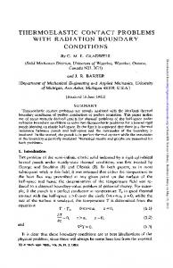
Table 1. Number of poles, p, required to approximate Si, I < M, with S(T, M)