ISEF'99 - 9th International Symposium on Electromagnetic Fields in Electrical Engineering Pavia, Italy, September 23-25, 1999. Published in COMPEL, 19, 2 (2000), pp. 239-45.
MOST GENERAL 'NON-LOCAL' BOUNDARY CONDITIONS FOR THE MAXWELL EQUATIONS IN A BOUNDED REGION A. Bossavit EdF, 1 Av. Gal de Gaulle, 92141 Clamart, France,
[email protected]
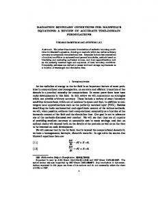
Introduction Setting up boundary conditions is probably the most difficult task in device modelling. Boundary conditions of the "n × H = something" kind, while easily implemented, don't cover all cases one may encounter. Users of commercial codes regularly report difficulties in specifying such obvious data as voltage drops, forced intensities, etc. The present paper attempts a classification of such boundary conditions, which we call "non-local" for want of a better and more universally adopted terminology. The main theoretical concept, which we aim at defining with workable definiteness, is impedance, for a device with a finite number of ports of entry. Considerations of software engineering are the main issue here. When designing a computing code, one must make provisions for all reasonable possibilities (and for some unreasonable ones). There are two methods: the extensive approach, which tries to list out all desired "features" and all "cases" that should be solvable, and the comprehensive one, in which some abstract representation of the category of problems one wants to solve will generate, by top-down development, an orderly code structure. The present paper is in the spirit of the latter approach. It is, however, very preliminary, as other issues than boundary conditions would need attention from the above viewpoint, which are not addressed here. We also ignore non-homogeneous local conditions, including so-called "absorbing" ones. Our main concern is with topological features: presence of loops, holes, and connectedness, or lack of it, of parts of the boundary subject to different conditions. The right tool for this is homology, which will openly be used. We don't assume any previous knowledge of it, and provide all needed definitions, but don't indulge in featherbedding either. Experienced programmers know well that only by using the abstract style of mathematics can one approach the exacting precision required in drafting program specifications. (Our goal, however, is to take advantage of mathematical facts, not to prove them; hence the substitution of pictures to formal reasoning.) Maxwell equations, a priori, concern the whole space. But in modelling, we have a specific region in view, most often. So we divide space into two parts: the computational domain, here denoted D, and the rest of the world, and we specify the influence of the latter by setting boundary conditions. Some freedom of choice goes into the definition of D, and most often, we may arrange things in such a way that its boundary S splits into three parts (none of which is necessarily in one piece): the "magnetic wall" S h, where n × H = 0, the "electric wall" Se , where n × E = 0, and the "no-flux, no-current" surface S e h, where n · rot E = 0 and n · rot H = 0 (i.e., n · B = 0, and n · J = 0 when displacement currents can be neglected). Connected components of S h and S e are the entry ports, between which voltage drops (emf's) or magnetomotive forces (mmf's) are applied, or through which currents, or magnetic fluxes, are forced. (Such ports are also, intuitively, the gates by which power enters the region of interest, although close examination of the Poynting theorem will partly refute this naive view.) The arch-simple example at the left of Fig. 1 may help rationalize the introduction of S h, Se , and S e h. The computational domain is a cylinder, enclosing a conductor. Current may have complex patterns in the middle, due to the change of section-shape, but is approximately vertical at both ends, hence n × E = 0 on the two "electric ports", forming Se , as shown. On the rest of the boundary, the magnetic field is approximately tangential, hence n · B = 0, and of course n · J = 0, so considering it as an S e h-surface is a valid approximation. There are no "magnetic ports", but an Sh-surface, lying in plane Σ, will appear if one takes advantage of symmetry to cut the domain in half. (Then D will not correspond to the original configuration, only to a part of it.) Many other examples will come to mind, where the S = Se ∪ Sh ∪ Se h splitting is similarly natural.
However, we shall rather reason on the more abstract example displayed on the right, which is the simplest case with enough generality: two ports of each kind, and one "loop" in the computational domain. The surface paths shown, which either link subparts of S e or Sh, or go around them, are dubbed "e-cycles" (here c i , i = 1 to 4) and "h-cycles" (here c i , i = 1 to 4). Our main task will be to define these geometrical objects. For now, just observe that e-cycles and h-cycles are paired (c 1 and c 2 count twice, so to speak, c 1 being c 2, and c 2 being c1 run along the other way), with transverse intersection, an essential property in what follows. E-cycles are oriented arbitrarily, and their mates have a matching orientation (to the right with respect to the e-cycle). The general idea is that emf's (resp., mmf's) are circulations of E along e-cycles (resp. of H along h-cycles). e S Ÿ
Ÿ
eh
∑
S
h
c4
S
D
~ c4
eh
S
c1
C
c2 , ~c 1 D c1, – c~2
J
~ c1
Ÿ
e
S c3
e
S
h
S S
e
~c 3
Fig. 1. Left: a common simple case (conductor C inside domain D). Right: a more abstract, general enough, example (inner conductors not shown). Theory 1
Let D, with boundary S, be a regular bounded open region, connected but not necessarily simply connected, in dimension 3. The system of equations we address is, for a given p ∈ C (p = ξ + iω , with ξ ≥ 0), −pε
E
+ rot
H
= J,
pµ
H
+ rot E = 0,
(1)
where fields are complex-valued, plus boundary conditions n×
E
= 0 on Se , n ×
H
= 0 on Sh, n · rot E = 0 and n · rot H = 0 on Se h,
(2)
and J given (source-current). The system comes from Maxwell’s time-domain formulation via Laplace transform, so its study covers all situations with linear constitutive laws. The well known harmonic case is when p = iω. The system has more generality than it seems, for ε and µ can be complex-valued: ε = ε' − i ε'', µ = µ' − i µ'', with ε', ε'', µ', µ'' all ≥ 0. In particular, one gets the eddy-currents problem, as formulated after Laplace transform, by simply setting ε = σ/p, σ > 0. We deal here with the case where all sources of the field are at the boundary, so J = 0 in (1). (To the extent that we are only interested in boundary conditions here, this is not a severe restriction.) It is then clear that (1)(2) are not enough to determine the fields: we need "non-local" boundary conditions, which we shall now introduce, beginning with some elements of homology. Let’s call paths, or smooth trajectories in S, the piecewise smooth (differentiable) mappings from [0, 1] into S. The reverse – γ of a path γ is the trajectory t → γ (1 − t). (Two distinct trajectories with the same image in S, like for instance γ and – γ , are not the same path.) The null path is obtained when γ (t) is some fixed point x, the same for all t. A 0-chain (with signed integer coefficients), denoted c = ∑ i zi xi , is a formal sum of points (each point x i being taken with the "weight" zi ). The boundary of a path γ is the 0-chain γ (1) – γ (0), and is denoted ∂γ . A 1-chain, denoted c = ∑i zi γ i , is a formal sum of paths. (One can see it as "γ 1 traversed z1 times (or, if z1 is negative, − γ 1 traversed |z 1| times), γ 2 traversed z2 times, etc.", all that in any order. Most chains we consider in the sequel are actually based on a single path, i.e., there is only one i, 1
Boundedness is not essential, and regularity can be relaxed to a large extent. "Piecewise smoothness" is enough.
and zi = ± 1.) Chains can be added: the sum of c = ∑ i zi γ i and c' = ∑ i z'i γ i is ∑ i (zi + z'i ) γ i , and multiplied by an integer. The null chain obtains when all z i 's are 0, or when each γ i is a null path. Of course we write c = c' if c – c' is a null chain, and we consider all null chains as one and the same, denoted 0. (Don't confuse 0-chains with the null chain!) The boundary of the 1-chain c = ∑ i zi γ i is by definition the 0-chain ∂c = ∑i zi ∂γ i . Similarly, 2-chains are formal sums of continuous images of the unit square ("patches"), and their boundaries are sums of images of the four segments of its boundary. A chain is a cycle if its boundary is the null chain. Remark that the boundary of a boundary is always the null chain: ∂∂c = 0, if one agrees that the boundary of a point is zero. Hence all boundaries are cycles. But the converse is not true (cycles c1 and c 2 on Fig. 1 don't bound). Two p-chains c and c' are homologous if c − c' is the boundary of some (p + 1)-chain, and we denote this by c ~ c'. In particular, if c is a boundary, then c ~ 0. Examples (p = 1): c 3 on Fig. 1 is homologous to 0, but c1 is not; c4 is homologous to the rim of the upper part of Sh. Ÿ
Next, let’s restrict to chains the elements of which (points, paths, patches) are all contained in Se h . The relative boundary, or boundary modulo Sh (resp. S e ) is what one gets by substituting 0 to the weights of all elements of the boundary that belong to Sh [resp. to Se ]. A chain is a relative cycle, or a cycle mod. Sh (resp. S e ) if its relative boundary is the null chain. On Fig. 1, c1 and c2 are cycles mod. S e , and also mod. S h (let's call these "absolute" cycles), c3 is a cycle only mod. Se , and c 4 is one mod. S h only. Two p-chains c and c' are homologous modulo Sh or S e if c − c' is the relative boundary of some (p + 1)-chain. One denotes this "c 1 ∼ c2 mod. S h (or Se )". For instance, on Fig. 1, c4 ~ 0 mod. S h: indeed, the collar above c4 can be dissected into patches, and thus is the image of some 2-chain in Se h , the relative boundary of which is c4. But c4 is not ~ 0 modulo Se . Ÿ
h
h h e
e
e
h
e h
e
e
h
h
e
e h e
h e
h
Fig. 2. A systematic, if not altogether elegant way to pair e-cycles and h-cycles. So what is special with the cycles sketched on Fig. 1? This: Our "e-cycles" are selected in order to form a basis for all cycles mod. S e , in the sense that, if a cycle c is not a relative boundary, then c ~ ∑ i = 1, ..., 4 zi ci for some coefficients z i , not all zero. Same thing about the "h-cycles". Fig. 1 suggests that e-cycles and h-cycles go by pairs: to each of a kind, c i , corresponds one of the other kind, c i , that intersects it (is “transverse” to it), and intersects no other. This is general, for as Fig. 2 demonstrates, one may always select basis elements this way: First, since connected components of S e h can be treated independently, one may assume Se h connected. Second (by general results of surface theory [1]), S e h is homeomorphic to a disk equipped with "handles" (one for each "loop"), as suggested by Fig. 2, left. (This way of sewing up handles is right for an orientable surface, which S e h necessarily is.) Finally, the boundary of Se h is made of closed curves, in finite number, each of which can be cut into successive curved segments, belonging to S e and S h in alternation. Fig. 2, right, shows how to join such segments by paths, in order to obtain a basis of relative cycles of each kind, with unique pairing. Absolute cycles, going two by two (and doing double duty, as above), can be added independently, one pair for each loop. (One such pair is sketched on Fig. 2, way up in the domain. It's the handle of the left, as seen from above.) E-cycles are oriented arbitrarily, and orientations of the h-cycles follow (each has its e-mate "going leftwards" at the crossing point, if the outward normal to S is supposed to point towards us). Note the change of sign this necessarily implies in the case of absolute cycles (c 2 = – c1 on Fig. 1). Ÿ
Ÿ
We denote the e- and h-cycles by ci and c i respectively, i spanning an index set I with |I| elements (|I| = 1 and 4 in the cases of Fig.1, left and right). Ÿ
Next, let's define functional spaces. We work in Euclidean space E3 with dot-product ' · '. A complex 3D-vector U is written U = uR + iuI, where uR and u I are real, and we extend the dot-product to complex vectors by setting U · V = uR · v R – uI · vI + i(uR · vI + uI · v R). The scalar product of two complex-valued fields defined over a domain D is then (U, V) = ∫D U(x) · V(x)* dx, where * denotes conjugation. The Hilbert space generated by fields with finite ( U, U) is denoted L2(D), like the space of square-summable scalar fields (with no serious risk of confusion). Then L2rot(D) = {U ∈ L2(D) : rot U ∈ L2(D)}. Notations HS, ES, etc., refer to the tangential parts of fields, n is the outward normal, grad S, rotS and divS are the differential operators acting on surface fields. The integral ∫c τ · U is the circulation of field U along circuit c, as equipped with its own field τ of unitary tangent vectors. Let us set E = {E ∈ L2rot(D) : n ×
E
= 0 on Se , n · rot
H = {H ∈ L2rot(D) : n ×
H
= 0 on Sh, n · rot
E
= 0 on Se h},
H
= 0 on Se h},
and introduce the continuous linear functionals V i (E) = ∫c i τ · E and Ji (H) = ∫c i τ · H. We denote by {V (E), J (H)} the vector formed by these quantities, an element of the complex vector space C2|I|. The following Lemma (which relies on a deep result of topology, the de Rham theorem) is the cornerstone of the theory: Ÿ
Lemma: If
E
∈ E and
H
∈ H, then ∫S n · (E × H) = – ∑ i ∈ I V i (E) Ji (H).
Proof. Set ES = – grad SΨ and HS = grad SΦ, using "cuts" along some cycles to make Φ and Ψ univalued if needed, and integrate by parts, using the formulas n · rot U = rotSUS and divS(n × US) = − rotSUS. ◊ It should be intuitively clear (think of the example of Fig. 1, left) that |I| of the 2|I| "non-local boundary data" V i (E) and Ji (H) should be specified in order to get a unique solution. More generally, let be given an affine subspace Γd of (complex) dimension |I| of C2|I| (d connotes "data"), and let us set EdH = {{E, H} ∈ E × H : {V (E), J (H)} ∈ Γd}, E0H = {{E, H} ∈ E × H : {V (E), J (H)} ∈ Γ0}, where Γ0 is the vector subspace parallel to Γd. (In practice, Γd will often be of the form Γd = {{V, J} ∈ C2|I| : V + Z J = E}, where Z is an |I| × |I| complex matrix—the "impedance of the outer circuit"—and E ∈ C|I| a given vector of complex outside emf's.) The non-local conditions we needed are then expressed by the clause {E, H} ∈ EdH,
(3) d
hence a precise weak formulation of problem (1)(2)(3), as follows: find a pair {E, H} ∈ E H such that p[∫D ε
E
· E' + ∫D µ
H
· H'] + ∫D rot E · H' – ∫D rot H · E' = 0 ∀ {E', H'} ∈ E0H.
(4)
(Beware, no complex conjugation.) Existence and uniqueness stem from the Lax–Milgram lemma, if one assumes ξ > 0. Implementation of this symmetrical formulation is straightforward with the primal- and dual-mesh technique exposed in [2]. Alternatively, one may eliminate either H or E from (4), using (1), and hence fall back on more familiar formulations. An important case in point is when all mmf's Ji are imposed. Call J the vector they form. (If i corresponds to an electric port, Ji is the "forced current" through it, in the eddy-currents interpretation.) Then (integrate by parts, and use the Lemma), pb. (4) rewrites as find E in E such that p ∫D ε
E
· E' + ∫D (pµ)–1 rot E · rot E' = ∑ i Ji V i (E') ∀ E' ∈ E.
(5)
Solving (5), using edge elements for E, one finds the vector V of emf's (a simple sum of edge-DoF's for each V i (E)), hence a matrix Z, depending on p, such that V = ZJ. This matrix is the (so-called "operational") impedance of the system, "as seen from" its electric and magnetic ports. Coupling with the outside world, then, simply amounts to solving (Z + Z)J = E. References [1] P.A. Firby, C.F. Gardiner, Surface Topology, Chichester: Ellis Horwood, 1982. [2] A. Bossavit, L. Kettunen: "Yee-like schemes on a tetrahedral mesh, with diagonal lumping", Int. J. Numer. Modelling (ENDF), 12 (1999), pp. 129-42.