method on dynamic mixed-model applications and show that run-time and ... actors represent computation while edges represents a FIFO communication ... For example, consider the Switch actor and the four SDF actors in Figure 1. ... Signal Proc. Image/Video. Comm Sys. Meta-Modeling. PDF. BLDF. Dynamic. CFDF. BDF.
A Generalized Scheduling Approach for Dynamic Dataflow Applications William Plishker, Nimish Sane, Shuvra S. Bhattacharyya Electrical and Computer Engineering Department University of Maryland College Park, Maryland, USA {plishker, nsane, ssb}@umd.edu
Abstract—For a number of years, dataflow concepts have provided designers of digital signal processing systems with environments capable of expressing high-level software architectures as well as low-level, performance-oriented kernels. But analysis of system-level trade-offs has been inhibited by the diversity of models and the dynamic nature of modern dataflow applications. To facilitate design space exploration for software implementations of heterogeneous dataflow applications, developers need tools capable of deeply analyzing and optimizing the application. To this end, we present a new scheduling approach that leverages a recently proposed general model of dynamic dataflow called core functional dataflow (CFDF). CFDF supports high-level application descriptions with multiple models of dataflow by structuring actors with sets of modes that represent fixed behaviors. In this work we show that by decomposing a dynamic dataflow graph as directed by its modes, we can derive a set of static dataflow graphs that interact dynamically. This enables designers to readily experiment with existing dataflow model specific scheduling techniques to all or some parts of the application while applying custom schedulers to others. We demonstrate this generalized dataflow scheduling method on dynamic mixed-model applications and show that run-time and buffer sizes significantly improve compared to a baseline dynamic dataflow scheduler and simulator.
I. I NTRODUCTION For a number of years, dataflow models have proven invaluable for application areas such as digital signal processing (DSP). Their graph-based formalisms allow natural and yet semantically rigorous application descriptions. Such a semantic foundation enables a variety of analysis tools, including determining buffer bounds and efficient scheduling [1]. As a result, dataflow languages are increasingly popular. Their diversity, portability, and intuitive appeal have extended them to many application areas with a variety of targets. (e.g., see [2] [3]). As system complexity and the diversity of components in digital signal processing platforms increases, designers are expressing more types of behavior in dataflow languages, even combining different dataflow models to describe a single application. While the semantic range of DSP-oriented dataflow models has expanded to cover dynamic interactions, dealing with model heterogeneity of dataflow is still cumbersome. This is especially problematic in scheduling, which has a major impact on key implementation metrics for embedded software systems, including memory size, performance, and power consumption (e.g., see [4]). Since scheduling techniques are
978-3-9810801-5-5/DATE09 © 2009 EDAA
model specific, designers are often forced to structure their applications for existing schedulers. Ideally, designers would need to only focus on describing functionality without implementation considerations. An automated tool would extract those parts of the application available for optimization, considering multiple dataflow models. Specific optimization techniques could be applied to relevant parts of the application, making this step independent from the functional description of the application. A designer could try different schedulers with different compilers or software synthesis techniques, giving the designer a fast iterative design framework for improving the resulting software implementation. To move towards this design flow, we propose a new scheduling approach that may be applied to dynamic heterogeneous applications. We leverage an existing design flow based on the dataflow interchange format (DIF) package [5], which was recently extended to include capabilities for the functional simulation of heterogeneous applications. These capabilities for functional simulation in DIF are provided through a framework called functional DIF [6]. Functional DIF supports dynamic dataflow applications with a semantic model called core function dataflow (CFDF), which enables dynamic behavior through structured application descriptions, making it an ideal platform to demonstrate a generalized scheduling approach. In this paper, we present an algorithm that takes dynamic applications described in the functional DIF formalism and decomposes the application into a set of static dataflow graphs. Existing scheduling techniques can then be applied to these static dataflow graphs. These statically-scheduled subgraphs dynamically interact to produce the original application behavior. Designers using this approach are able to arrive at quality implementations of dynamic, heterogeneous dataflowbased systems quickly. This paper has the following sections: Section 2 discusses related background, while Section 3 surveys related research to place this work in context. Section 4 describes our approach to generalized scheduling, and Section 5 demonstrates it on a representative set of applications.
TABLE I T HE BEHAVIOR OF MODES IN ACTOR S WITCH
� Ϯ ϭ
�
Ϯ
ϭ
^ǁŝƚĐŚ
ϭ͕Ϭ
ϯ
Ϭ͕ϭ
ϭ
� �
^ǁŝƚĐŚ �ŽŶƚƌŽů� DŽĚĞ dƌƵĞ� DŽĚĞ
&ĂůƐĞ� DŽĚĞ
mode Control True False
consumes Control Data 1 0 0 1 0 1
produces True False 0 0 1 0 0 1
output, respectively. While each mode has fixed production and consumption behavior, the dynamic nature of Switch is captured by transitions between the modes shown in Figure 1 as mode transition edges. B. Dataflow Interchange Format
Fig. 1.
Boolean dataflow switch described in CFDF.
II. BACKGROUND A. Dataflow Modeling Modeling DSP applications through coarse-grain dataflow graphs is widespread in the DSP design community, and a variety of dataflow models have been developed for dataflowbased design. A growing set of DSP design tools support such dataflow semantics [7] [8]. Designers are expected to be able to find a match between their application and one of the wellstudied models, including cyclo-static dataflow (CSDF) [9], synchronous dataflow (SDF) [1], single-rate dataflow, homogeneous synchronous dataflow (HSDF), or a more complicated model such as boolean dataflow (BDF) [10]. Common to each of these modeling paradigms is the representation of computational behavior as a dataflow graph. A dataflow graph G is an ordered pair (V, E) , where V is a set of vertices (or nodes), and E is a set of directed edges. A directed edge e = (v1 , v2 ) ∈ E is an ordered pair of a source vertex v1 ∈ V and a sink vertex v2 ∈ V . Nodes or actors represent computation while edges represents a FIFO communication links between them. The semantic foundation for functional DIF is core functional dataflow (CFDF) [6], which is capable of expressing deterministic, dynamic dataflow applications. In this formalism, each actor a ∈ V has a set of modes, Ma , in which it can execute. Each mode, when executed, consumes and produces a fixed number of tokens. Each actor a ∈ V has an enabling function which indicates if a given mode may be executed given the present state of the application. The invoking function for an actor a takes an enabled mode and executes the associated computation, consuming and producing tokens. The invoking function of an actor can change the mode of execution of the actor, so the invoking function also produces the next mode that is valid. For example, consider the Switch actor and the four SDF actors in Figure 1. SDF actors can be described with only one mode, but the Switch is described with 3 modes as shown in Table I. In the mode Control one control token is read, while in True or False the data token is routed to the true or false
To describe the dataflow applications for this wide range of dataflow models, application developers can use the dataflow interchange format (DIF) [5], an approach founded in dataflow semantics and tailored for DSP system design. The DIF language (TDL) provides an integrated set of syntactic and semantic features that can fully capture essential modeling information of DSP applications without over-specification. From a dataflow point of view, TDL is designed to describe mixed-grain graph topologies and hierarchies as well as to specify dataflow-related and actor-specific information. The dataflow semantic specification is based on dataflow modeling theory and independent of any design tool. To utilize the DIF language, the DIF package (TDP) has been built. Along with the ability to transform DIF descriptions into a manipulable internal representation, TDP contains graph utilities, optimization engines, algorithms that may prove useful properties of the application, and a C synthesis framework [11]. These facilities make the DIF package an effective environment for modeling dataflow applications, providing interoperability with other design environments, and developing new tools. An overview of the DIF design flow using TDP is shown in Figure 2. Beyond these features, TDP is also suitable as a design environment for implementing dataflow-based application representations. Describing an application graph is done by listing nodes and edges, and then annotating dataflow specific information. TDP also has an infrastructure for porting applications from other dataflow tools to DIF. The ability to simulate functional designs in TDP has been recently added, but like other dynamic dataflow design tools, TDP has been missing a scheduling approach for dynamic applications. III. R ELATED W ORK A number of development environments utilize dataflow models to aid in the capture and optimization of mixed-model applications. Ptolemy II encompasses a diversity of datafloworiented and other kinds of models of computation [12]. Developers employ a “director” that controls the communication and execution schedule of an associated application graph. To describe an application with multiple models of computation, developers can insert a “composite actor” that represents a subgraph operating with a different model of computation
Dataflow Models
Static SDF
MDSDF
HSDF
CSDF
Dynamic CFDF
DSP Designs
BDF
PDF
The DIF Language (TDL)
DIF Specification
The DIF Package (TDP)
Front-end
AIF / Porting
Embedded Processing Platforms
BLDF
Image/Video Comm Sys
Algorithms
DIF-to-C DIF Representation
Ptolemy Ex/Im
Dataflowbased DSP Design Tools
Signal Proc
Meta-Modeling
DIF-A T Ex/Im
Ptolemy II
Autocoding Toolset
Java
Ada
Java VM
VDM
Fig. 2.
Other Ex/Im
DSP Libraries VSIPL
Other Tools TI
Other Embedded Platforms
Other
C DSP
DIF based design flow
(and therefore its own director). In such hierarchical representations, directors manage the actors only at their associated design levels, and directors of composite actors only invoke their actors when higher level directors execute the composite actors. A domain-specific example of targeting actor descriptions is CAL [13]. CAL has a variety of language constructs including actions, guards, variables, and expressions. CAL is rooted in a semantic formalism, but for the sake of portability and ease of use, it uses a minimal semantic core. The SysteMoC approach employs SystemC to capture actors as composed of input ports, output ports, functionality, and an execution FSM, which determines the communication behavior of the actor [14]. SysteMoC also facilitates the mapping of application graphs to architecture graphs. For complete functionality in Simulink [8], actors are described in the form of “S-functions.” By describing them in a specific format, such actors can be used in continuous, discrete time, and hybrid systems. In the Stream Based Function (SBF) model of computation [15], actors are represented by a set of functions, a controller, state, and transition function. Each function is sequentially enabled by the controller, and uses blocking reads to consume a single token from its inputs. Once a function is done, the transition function defines the next function in the set to be enabled. Our generalized scheduling framework differs from these related efforts in dataflow-based design in that our framework uses top-down analysis of (explicitly-specified) application structure combined with integration of static dataflow subbehaviors (actor modes) across groups of dataflow actors. This approach to analysis and integration systematically extends the reach of static scheduling techniques so that they can be used across significant portions of dynamic dataflow designs. The approach is driven by the modeling architecture of functional DIF, which provides the explicit decomposition of actors into static dataflow sub-behaviors, and efficiently exposes to the scheduler the design spaces associated with separating subbehaviors of individual actors, and grouping subsets of subbehaviors across different actors. A limitation of our approach, compared to related tech-
niques, is that special attention is required by the designer to explicitly specify the dataflow properties associated with individual modes, and attention is also needed during testing to validate that the declared and observed behaviors match. An interesting direction for future work is the integration of our proposed scheduling methods with more formal reasoning about actor sub-behaviors, such as those being developed in conjunction with languages and models such as CAL and SysteMoc. IV. G ENERALIZED DATAFLOW S CHEDULING A. Generalized Schedule Trees There are many types of schedulers and optimization routines that can the be applied to specific dataflow models (e.g., [16]), but scheduling commonalities exists across models. We leverage generalized schedule trees (GSTs) as a unifying schedule representation [17]. The GST representation in conjunction with CFDF semantics is well-suited for mixedmodel scheduling because it can be used to represent dataflow graph schedules irrespective of the underlying dataflow model or scheduling strategy being used. GSTs are ordered trees with leaf nodes representing the actors of an associated dataflow graph. An internal node of the GST represents the loop count of a schedule loop (an iteration construct to be applied when executing the schedule) that is rooted at that internal node. The ordering of leaf nodes determines the order in which actors of the application graph are traversed. Functional simulation of an application can be done by traversing an associated GST iteratively and checking for enabled actors (and then executing them, if appropriate) that correspond to the schedule tree leaf nodes. Note that if actors are not enabled, the GST traversal simply skips their invocation. Subsequent schedule rounds will revisit actors that were unable to execute in the current round. Having the ability to use a schedule tree in which we can safely “skip” (bypass invocation of) actors is well suited to dynamic applications, which is what we focus on in this work. B. Dynamic Dataflow Graph Decomposition To decompose a dynamic dataflow graph into a set of static interacting graphs, we utilize the fact that every mode has fixed production and consumption behavior. To construct a static graph based on these modes, we find the combination of modes in which one mode from each actor in the subgraph is producing or consuming on an edge that has a consuming or producing mode at the other end of the edge. Since every actor can potentially provide many modes, there are an exponential number of combinations to be considered. To limit the space explored, we perform a reachability analysis to consider only those modes that are connected to each other. To this end, we extend depth first search (DFS) graph traversal with the concept of mode traversal to arrive at the set of static subgraphs as shown in Figure 3. The key addition to the traditional DFS is that the next nodes to be added to the working stack S are found by following a mode from the current node. Another stack of nodes T keeps
�
DecomposeCFDFGraph(CFDFGraph G) Returns set of static graphs Graphs Gs ← {} for all source mode ∈ G do {use stacks for both the DFS and mode coverage } Stack S ← {}, Stack T ← {} mark every mode and node as not visited SDFGraph sdf G ← empty graph mark all other modes in node that contains source mode T .push(node that contains the source mode) while T has elements do S.push(T .pop()) while S has elements do Actor A ← S.pop() if A not visited then mark A as visited for all mode M ∈ A do if M not visited and matches the connecting edge then S.push(actors on inputs and outputs of M ) sdf G.add(A) sdf G.annInEdges(M .cons) sdf G.annOutEdges(M .prod) break forall end if mark M as visited end for if no matching mode found in A then {graph sdf G is invalid} break while end if T .push(A) end if end while {when the stack is empty, one static graph is complete} if sdf G is a valid and Gs.doesNotContain(sdf G) then Gs.add(sdf G) end if {in every case, unwind graph} while T has elements do if T.peek().allModesVisited() then Actor B ← T .pop() B.resetNodeVisitedFlag() B.resetAllModeVisitedFlags() else T .peek().resetNodeVisitedFlag() break while end if end while reset S using active edges from nodes in T end while end for Return Gs Fig. 3.
Algorithm for dynamic graph decomposition.
Ϯ ϭ
^ǁŝƚĐŚĐŽŶƚƌŽů �
Ϯ
ϭ
�
Ϯ
ϭ
Fig. 4.
^ǁŝƚĐŚƚƌƵĞ ^ǁŝƚĐŚĨĂůƐĞ
ϭ
ϯ
�
ϭ
ϭ
�
Application decomposition example
track of what order the nodes have been visited, so that the graph visited state may be unwound. When a static subgraph has been completed or an invalid graph has been found in the course of DFS, nodes are popped off of T until a node is found that has another mode to be considered (i.e. the potential of another unique static subgraph). Each of the popped nodes have their mode and node visited flags cleared, thus unwinding the graph state by making them available for the mode at the top of T . Therefore multiple graphs maybe constructed from the same source mode. For this paper, we only consider directed acyclic graphs, so DFS is started at the source modes in the application (i.e., those that do not need input tokens to execute). Note that mode transition edges are not considered as edges to be traversed in DFS, effectively separating the graph at mode boundaries. For example, consider the decomposition that results from Figure 1 as shown in Figure 4. Two source modes were found in A and B. The DFS from the mode of A ended immediately in the control mode of Switch, but the DFS from B found two matching modes in Switch (namely true and false). One state is taken, and a complete static graph is formed by following one of the branches. After the completed graph is saved from B, the graph visited state unwinds back to Switch and DFS continues using the remaining mode from Switch mode. Thus, the single dynamic BDF application graph has been transformed into three static subgraphs. Note that for a complete iteration of the original application to finish, more than one of the subgraphs must be run to completion. Indeed, because mode transitions may be arbitrary, we have no a priori way in general of exactly balancing the execution of these three graphs, and we must rely on the dynamic GSTs as described in Section IV-A for proper simulation. All graphs in the set of graphs that are created by this algorithm must be subgraphs of the original graph. Edges of this subgraph are annotated with the corresponding production and consumption numbers described by the modes used in a given run of DFS. Since the decomposition algorithm is based on DFS, the complexity of this algorithm is founded on it as well, but mode combinations make it exponential in the number of modes. Fortunately, we have found in practice that this approach is efficient, since modes tend to be connected together in a structured way.
TABLE II S IMULATION TIMES AND MAXIMUM BUFFER SIZES FOR MIXED - MODEL
/E
APPLICATIONS
ϭ ϭ
�/^dZ/�hdKZ ϭ
ϭ͕Ϭ
ĐĚϮĚĂƚϭͺĂ ϭ ϰ
ĐĚϮĚĂƚϭͺď ϳ ϱ
ϭ
ĐĚϮĚĂƚϮͺĂ ϭ ϭ
PolyPhase
Ϯ ϯ
Multi-PEA
ĐĚϮĚĂƚϮͺď
ĐĚϮĚĂƚϭͺĐ
ĐĚϮĚĂƚϮͺĐ
ĐĚϮĚĂƚϭͺĚ
ĐĚϮĚĂƚϮͺĚ
ĐĚϮĚĂƚϭͺĞ
ĐĚϮĚĂƚϮͺĞ
ĐĚϮĚĂƚϭͺĨ
ĐĚϮĚĂƚϮͺĨ
KhdWhdϭ
KhdWhdϮ
ϳ ϰ ϯ Ϯ ϭ ϭ ϭ ϭ
Fig. 5.
Ϭ͕ϭ
Application Sample Rate Conv
ϰ ϳ ϱ ϳ ϰ ϭ ϭ ϭ
Dual sample rate conversion application graph
V. R ESULTS To demonstrate this approach, we chose representative mixed-model applications to experiment with: a dynamic data distribution of audio streams to be sample-rate-converted, a polyphase decimated DFTfilter bank, and an application with multiple polynomial evaluation accelerators. Figure 5 shows a pictorial representation of the sample rate conversion application based on concepts found in [18] and [11]. Two audio channels are to be converted on two different subsystems. The input streams are interleaved, such as how multiple audio channels might come over a single digital input. With an arbitrary interleaving, the DISTRIBUTOR actor distributes them to the appropriate multirate datapath. In this case, a series of FIR filters is dedicated to sample rate conversion and the DISTRIBUTOR two modes that service arbitrary interleaving of the data. We also implemented an M channel uniform discrete Fourier transform (DFT) filter bank. We constructed a decimated uniform DFT filter bank using a mixed-model consisting of CSDF and SDF actors. In addition, to show the applicability of our approach to heterogeneous applications, we used one with multiple polynomial evaluation accelerators (PEAs), which utilizes both CSDF, SDF, and BDF elements [19]. Polynomial functions may change when senders transmit data to receivers, so the application employs Switch and Select to dynamically change between the two datapaths. Polynomial evaluation is a commonly-used primitive in various domains of signal processing, such as wireless communications and
Schedule Strategy Canonical Flat APGAN Canonical Flat APGAN Canonical Flat APGAN
Average Simulation Time (ms) 9,148 1,425 1,462 910 1,017 1,117 2,163 586 548
Max Observed buffer size (tokens) 9,394 2,408 2,278 17 24 24 11,198 57 57
cryptography. We applied our generalized scheduling approach to each of these applications and compared it to a naive round-robin scheduler called the canonical scheduler, in which every actor appears once in the schedule with a loop count of one. We compared this to the static subgraphs generated by our approach, which were scheduled with both a flat scheduler based on the repetition vectors of the SDF clusters and an APGAN-based scheduler [16]. The resulting schedule trees were combined into a single tree by profiling the number successful executions, to balance the execution rates. As an example, Figure 6 shows the APGAN-generated schedule derived from our design flow on the sample rate conversion application. Two unique schedule trees resulted from the two subgraphs from the original application, which were were evenly balanced based on profiling results. While at any given time the simulator might be traversing the wrong side of the schedule tree during execution, the guarded execution of checking the enabling function before invoking ensures the application produced correct results. Results for these different styles of implementation with different schedules are summarized by Table II. We simulated thousands of tokens for each application on a 1.7GHz Pentium with 1GB of memory. In two out of the three cases, utilizing the generalized scheduling technique produced a significant improvement in simulation time and buffer size needed. However, while the PolyPhase application has multiple static subgraphs, these subgraphs are not multirate, so the scheduler provides little benefit. Instead the lightweight canonical schedule better services this application. The diversity in results show the utility of being able to apply the generalized scheduling approach presented in this work. VI. C ONCLUSION In this work, we presented a new approach to scheduling dynamic dataflow applications. It leverages a new model of dataflow that structures dynamic actors as a set of modes with fixed behavior. We presented an algorithm that decomposes dynamic dataflow graphs into a set of dynamically interacting static dataflow graphs. We demonstrated this on mixed-model applications leveragin existing static schedulers, which gave a positive indication of the utility of this approach for software
1
20
1
IN
1
4
1
1
cd2dat1_B
1
1
7
49
4
cd2dat1_C
cd2dat1_A
7
3
1
2
cd2dat1_D
DISTRIBUTOR
cd2dat1_E
1
1
1
1
IN
OUTPUT1
1
DISTRIBUTOR
1
cd2dat2_A
8
2
cd2dat2_C
7
5
cd2dat2_D
1
1
cd2dat2_B
cd2dat2_E
4
1
cd2dat2_F
1
OUTPUT2
cd2dat1_F
Fig. 6.
The APGAN schedule of the sample rate conversion application
implementations of such dynamic dataflow applications. An immediate direction of future work is to improve the sophistication of the simulator. With a more intelligent way of dynamically switching between the resulting static schedule trees, we should achieve better runtimes and smaller maximum buffer sizes. Beyond that we would like to compare versus other dynamic scheduling approaches and to try more complex, real world applications, which we believe will further show the utility of this approach. ACKNOWLEDGMENTS This research was sponsored in part by the U.S. National Science Foundation (Grant number 0325119), and the US Army Research Office (Contract number TCN07108, administered through Battelle-Scientific Services Program). R EFERENCES [1] E. A. Lee and D. G. Messerschmitt, “Static scheduling of synchronous dataflow programs for digital signal processing,” IEEE Transactions on Computers, February 1987. [2] C. Shen, W. Plishker, S. S. Bhattacharyya, and N. Goldsman, “An energy-driven design methodology for distributing DSP applications across wireless sensor networks,” in Proceedings of the IEEE Real-Time Systems Symposium, Tucson, Arizona, December 2007, pp. 214–223. [3] W. Plishker, “Automated mapping of domain specific languages to application specific multiprocessors,” Ph.D. dissertation, University of California, Berkeley, January 2006. [Online]. Available: http://www.gigascale.org/pubs/1138.html [4] S. Sriram and S. S. Bhattacharyya, Embedded Multiprocessors: Scheduling and Synchronization. Marcel Dekker, Inc., 2000. [5] C. Hsu, I. Corretjer, M. Ko., W. Plishker, and S. S. Bhattacharyya, “Dataflow interchange format: Language reference for DIF language version 1.0, users guide for DIF package version 1.0,” Institute for Advanced Computer Studies, University of Maryland at College Park, Tech. Rep. UMIACS-TR-2007-32, June 2007, also Computer Science Technical Report CS-TR-4871. [6] W. Plishker, N. Sane, M. Kiemb, K. Anand, and S. S. Bhattacharyya, “Functional DIF for rapid prototyping,” in Proceedings of the International Symposium on Rapid System Prototyping, Monterey, California, June 2008, pp. 17–23. [7] G. Johnson, LabVIEW Graphical Programming: Practical Applications in Instrumentation and Control. McGraw-Hill School Education Group, 1997. [8] Using Simulink, Version 3 ed., The MathWorks Inc., Jan 1999.
[9] G. Bilsen, M. Engels, R. Lauwereins, and J. A. Peperstraete, “Cyclostatic dataflow,” IEEE Transactions on Signal Processing, vol. 44, no. 2, pp. 397–408, February 1996. [10] J. T. Buck and E. A. Lee, “Scheduling dynamic dataflow graphs using the token flow model,” in In Proceedings of the International Conference on Acoustics, Speech, and Signal Processing, April 1993. [11] C. Hsu, M. Ko, and S. S. Bhattacharyya, “Software synthesis from the dataflow interchange format,” in Proceedings of the International Workshop on Software and Compilers for Embedded Systems, Dallas, Texas, September 2005, pp. 37–49. [12] J. Eker, J. Janneck, E. A. Lee, J. Liu, X. Liu, J. Ludvig, S. Neuendorffer, S. R. Sachs, and Y. Xiong, “Taming heterogeneity - the Ptolemy approach,” Proceedings of the IEEE, Special Issue on Modeling and Design of Embedded Software, vol. 91, no. 1, pp. 127–144, January 2003. [Online]. Available: http://www.gigascale.org/pubs/393.html [13] J. Eker and J. Janneck, “Caltrop—language report (draft),” Electronics Research Lab, Department of Electrical Engineering and Computer Sciences, University of California at Berkeley California, Berkeley, CA, Technical Memorandum, 2002. [14] C. Haubelt, J. Falk, J. Keinert, T. Schlichter, M. Streub¨uhr, A. Deyhle, A. Hadert, and J. Teich, “A systemc-based design methodology for digital signal processing systems,” EURASIP J. Embedded Syst., vol. 2007, no. 1, pp. 15–15, 2007. [15] B. Kienhuis and E. F. Deprettere, “Modeling stream-based applications using the SBF model of computation,” in Proceedings of the IEEE Workshop on Signal Processing Systems, September 2001, pp. 385–394. [16] S. S. Bhattacharyya, P. K. Murthy, and E. A. Lee, Software Synthesis from Dataflow Graphs. Kluwer Academic Publishers, 1996. [17] M. Ko, C. Zissulescu, S. Puthenpurayil, S. S. Bhattacharyya, B. Kienhuis, and E. Deprettere, “Parameterized looped schedules for compact representation of execution sequences,” in Proceedings of the International Conference on Application Specific Systems, Architectures, and Processors, Steamboat Springs, Colorado, September 2006, pp. 223– 230. [18] J. Dalcolmo, R. Lauwereins, and M. Ade, “Code generation of data dominated DSP applications for FPGA targets,” in Proceedings of the International Workshop on Rapid System Prototyping, June 1998, pp. 162–167. [19] W. Plishker, N. Sane, M. Kiemb, and S. S. Bhattacharyya, “Heterogeneous design in functional DIF,” in Proceedings of the International Workshop on Systems, Architectures, Modeling, and Simulation, Samos, Greece, July 2008, pp. 157–166.