A Generic Framework for Continuous Motion Pattern Query Evaluation Petko Bakalov University of California Riverside, CA 92521
[email protected]
Vassilis J. Tsotras University of California Riverside, CA 92521
[email protected]
Abstract
static spatiotemporal archives like [11, 5] in two major aspects. First, the continuous nature of the streaming data requires real time processing using relatively simple data structures for indexing. Second, in the streaming environment the query evaluation is a continuous process. Unlike the typical snapshot queries over the static archives that are evaluated only once, continuous queries require a continuous reevaluation since results become obsolete and invalid as information about the monitored objects changes. Recent research in continuous spatial query processing has been focused mainly on single predicate queries, where the predicate is a Range [3, 12] or a Nearest Neighbor [6]. In this paper we focus on the continuous evaluation of “motion pattern” (i.e. CMP) queries. Here a single query is expressed with multiple predicates, correlated over time. We argue that since the data produced by the monitored moving objects is “trajectorial” in nature, users of these surveillance and tracking systems should also be able to query the “behavior” of the moving objects over time. Consider for instance a criminal offenders monitoring application (like tracNET24 or ExacuTrack) which tracks the movement of law offenders (through special wearable GPS devices) inside a given area and alerts the correctional officers for any suspicious or illegal behavior. The suspicious behavior can be defined as a CMP query like: “Continuously report objects that did pass through all five bank offices in the area and have been in areas not covered with surveillance cameras for more than 20 minutes in the last half an hour”. In this example, the object behavior is captured by the sequence of spatial (range) predicates ordered by time, where the temporal predicates are relative to the ever increasing current time. This type of query cannot be answered with processing methods focused only on the current state of the stream; rather, we need to maintain and query appropriate past states (the history) of the spatiotemporal stream. Motion pattern queries [4] have been well studied for static spatiotemporal archives (i.e., when all data is known in advance and the query is evaluated once). To the best of our knowledge there is no work for this problem in the
We introduce a novel query type defined over streaming moving object data, namely, the Continuous Motion Pattern (CMP) Queries. A motion pattern is defined as a sequence of distinct spatial predicates, each attached to a temporal constraint. The spatial predicates can be of various types (range, nearest neighbor, etc.) The temporal constraints are relative to the current time instant and are used to specify the order of the spatial predicates on the time axis. A CMP query is continuously reevaluated over streaming spatiotemporal data, producing the moving objects which satisfy the query’s motion pattern. We first introduce an easily maintainable indexing scheme for spatiotemporal streams that facilitates the evaluation of the spatial predicates over their temporal constraints. Using this scheme we propose a generic framework for efficiently answering a wide range of CMP queries. The effectiveness of our algorithms in reducing the query computation cost and I/O operations is revealed through a thorough experimental evaluation.
1 Introduction The widespread use of location detection devices (RFID, GPS etc.) has enabled the creation of complex tracking and situational awareness systems which continuously monitor the position of moving objects of interest and can thus provide complex services to their end users. Example applications include security monitoring, vehicle tracking, traffic management, etc. In a typical surveillance system architecture the set of monitored objects continuously report their position to the data collection device using data packets containing their identifier, current location and timestamp. These data packets are combined into a single spatiotemporal stream that is forwarded to a centralized server for query processing. The system users register their queries to the server and continuously receive the result based on the changing state of the data. The described streaming architecture differs from the 1
streaming environment where the query result has to be constantly reevaluated. A trivial solution involves repetitive execution of the static algorithms described in [4], i.e. every time when the result becomes obsolete it has to be recomputed. This would be very expensive and inefficient since in a typical streaming environment location updates are very frequent. The predominant approach for effective evaluation of continuous queries is by incremental processing [20, 19]. This strategy implies that the query processor utilizes as much as possible the current intermediate results and data structures in the successive iterations of the evaluation algorithm. The query result can be kept persistent during consecutive iterations by applying positive and negative updates on it. In this paper we first present a novel indexing scheme for answering CMP queries on spatiotemporal streams. Using this indexing structure we propose an efficient framework for incremental evaluation of a wide range of CMP queries. The effectiveness of our algorithms is revealed trough an extensive experimental evaluation.
tenance, a grid structure can handle very effectively issues like frequent updates, high arrival rates, and the continuous nature of the data, which are critical in a streaming environment. Unfortunately, because of its simplicity this structure cannot capture the temporal characteristics of the data and can be used only for a queries focused on the current state of the stream. Thus it cannot be used directly to evaluate continuous motion pattern queries. Methods using tree structures are either B+-tree based [9] or R-tree based [7, 8, 18, 16, 17]. The main objective here is to improve the index update performance. In [7] the amortized update cost is reduced by avoiding updates for objects that do not move outside their MBRs. [8] generalized this technique through a bottom - up update strategy. [9] propose instead the linearization of the moving object location representation by using space filling curves. Then B+ trees can be used, which have better update characteristics than R-trees. The last group [15, 10] of query evaluation methods for spatiotemporal streams avoids the expensive maintenance of index structures over the streaming data. Instead, they introduce the notion of safe regions, created either around the moving object [15] or around the query [10]. If the object does not leave its safe region no further query processing is required. Similarly in [10] objects are considered only if they fall inside the query region or its uncertainty regions.
2 Related Work With the exception of [4] which presents a set of algorithms for pattern query evaluation in a static environment, all previous related work on spatiotemporal pattern queries deals only with modeling and language issues. [1] proposes using spatiotemporal patterns as a systematic and scalable query mechanism to characterize complex object behaviors in space and time; nevertheless no query evaluation strategy is proposed. Similarly [13] presents a powerful query language able to describe complex pattern queries using a combination of logical functions and quantifiers. This language however is of declarative nature and cannot be used the query optimization. Pattern queries have recently attracted interest for a numerical (i.e no trajectory) data in a relational DBMS. Related to our research is also the work done on continuously querying spatiotemporal streams. Various indexing structures have been proposed in the past as well as multiple algorithms utilizing these structures to answer mainly NN and range queries. They all fall in three basic categories: (i) methods using grids, (ii) methods utilizing tree structures, and, (iii) methods using “safe” regions. Many of the proposed indexing structures [3, 14] use a simple grid to index the location of the objects inside the spatiotemporal stream. Every cell inside the grid structure keeps a list with the objects whose location is within the boundaries of this cell. Multiple algorithms have been proposed to solve single range [3, 12]. and NN predicates [6, 14]. using this simple grid structure in distributed and centralized environments. Given its straightforward main-
3 Problem Definition Consider a situational awareness system that continuously monitors the location of a set of moving objects. Location data arrive as a stream of tuples S ≡ hu1 , u2 , . . . , ul , . . .i where ui ≡ ho, l, ti, o is the moving object identifier, t is the observation timestamp and l is the object location at time t (where l ∈ Rd , t ∈ N, o ∈ N). A trajectory T R(oj , T ) of object oj inside the stream S for time predicate T is defined as a sequence of tuples u1 , u2 , . . . , un , . . . where ui .o = oj and ∀i , ui .t ∈ T . The notation used in the rest of the paper is summarized in the following table: Notation Q T oj CN P CBP
Meaning continuous spatial predicate relative time constraint spatial object set of continuous numerical predicates set of continuous binary predicates
Our definition of continuous motion pattern queries is based on the notion of pattern queries defined in [2]. However instead of absolute time constraints we use relative ones; in a streaming environment absolute time constraints as defined in [2] do not apply since their result never 2
a spatiotemporal stream S, f is a score function if f (Qi , T R(oj , Ti ), Ψi ) = c where c ∈ R for a numerical spatial predicate or c ∈ B for a binary spatial predicate. Given a pattern query Q and a stream S our goal is to find the moving objects oj ∈ S which satisfy the query Q. If the query Q contains binary predicates CBP we have to find all objects oj which satisfy all binary predicates (i.e. ∀Qi ∈ CBP → f (Qi , T R(oj , Ti ), Ψi ) = true). The binary predicates are aggregated using the operator ∩ (AND). If the query Q contains numerical predicates CN P , their scores on object oj are aggregated using a summation to produce an object numerical score µj .
changes. A relative time constraint uses the current time instance as a reference point. (e.g.. “between 40 and 50 minutes ago”). As time advances, the value of the current timestamp changes, forcing the relative time constraint slide along the temporal axis. More formally a CMP query Q is expressed as a sequence of (arbitrary number) n spatiotemporal predicates: Q = {(Q1 , hT1 , Ψ1 i), . . . , (Qn , hTn , Ψn i), Θ} where Qi is a spatial predicate, Ti is a relative time constraint, Ψi is a logical quantifier (Ψi ≡ {∀, ∃}) which indicates if the spatial predicate is applies for the whole duration of the time constraint Ti or just for one time instance. Θ is an operator that maps a real value R to a boolean B ≡ {true, f alse}. Note that in the definition above the temporal constraints Ti are optional. If there is no temporal constraint provided for spatial predicate Qi a temporal ordering is implied by the actual position of the predicate Qi in the query sequence Q. For example in the query:
X
µj =
f (Qi , T R(oj , Ti ), Ψi )
Qi ∈CN P
To determine if an object oj satisfies the CN P predicates of query Q its numerical score has to be mapped to a binary value. This is done by the Θ operator defined in the query Q. An example of Θ operator can be the simple check function “≤ 4”. In this example Θ will return true for all objects oj that have a sum of the numerical scoring functions less or equal than 4 (i.e., µj ≤ 4). It is also possible to use more sophisticated Θ operators like min or max. In the first case the operator will return true only for the object which has the smallest numerical score µj . In analogy Θ ≡ max will return true only for the object with the highest numerical score. To summarize, in order to check if an object oj satisfies Q we compute λ(Q, oj ) where:
Q = {(Q1 , (30, 20), ∀), (Q2 ), (Q3 ), (Q4 , (10, 5), ∃), Θ} defines a pattern where the spatial predicate Q1 is satisfied for every time instance in the time interval between 20 and 30 minutes ago, Q4 is satisfied for at least one time instance in the time interval between 5 and 10 minutes ago and the predicates Q2 and Q3 are satisfied between predicates Q1 and Q4 in that order. We allow a very general class of spatial predicates to participate in a CMP query. A spatial predicate Qi is described through a spatial object soi (where soi represents point or region) and can be either binary or numerical. Let CBP (respectively CN P ) denote the set of all binary (respectively, numerical) predicates. Binary spatial predicate: A predicate Qi ∈ CBP maps a combination between a moving object oj and the spatial object soi defined in this predicate to a boolean value B ≡ {true, f alse}. That is Qi ≡ oj × soi → B. An example of a binary predicate is the predicate Inside. that checks whether the moving object oj is inside region soi Range predicates belong to CBP as well. In analogy: Numerical spatial predicate: A predicate Qi ∈ CN P maps the combination of moving object oj and spatial object soi to a real value. That is oj × soi → R. A numerical spatial predicate example is the function min distance which returns the minimal distance between the moving object oj and spatial object soi (which can be a point or a region). Clearly NN predicates belong to CNP. For both binary and numerical predicates the mapping is done through a score function f (Qi , T R(oj , Ti ), Ψi ). Given a single spatial predicate Qi , its relative time constraint Ti , quantifier Ψi and a moving object oj in
λ(Q, oj ) ≡
\
f (Qi , T R(oj , Ti ), Ψi )
Qi ∈CBP
∩ Θ(
X
f (Qi , T R(oj , Ti ), Ψi ))
Qi ∈CN P
and λ ≡ {true, f alse}.
4 Index Structure Given that incremental processing has been shown to be the most efficient approach for continuous query evaluation, we need an appropriate spatiotemporal indexing structure that can accommodate positive and negative updates. Such structure should answer efficiently questions of the type “given area A, provide all objects that are not in A at the previous time instant but appear in A at the current instant” (a positive update), or, “provide all objects that do not appear in A in the current time instant but were in A at the previous one” (a negative update). Generating positive or negative updates every time an object changes its location would produce an intractable number of such updates. Instead we generate positive and 3
To Time 3
1
t2 Index Point 2
tto tfrom
t1
2
4
Index Point 1
tfrom 1
2
3
… … … …
t2
Data Pages
t1
tfrom
tto
Negative Updates (Region 2)
tfrom
tto
“Trough’ objects (Region 3)
tfrom
tto
“In-out’ objects (Region 4)
tfrom
tto
Figure 3. Indexing space projection.
Time From
t1
From Positive Updates (Region 1)
Figure 1. 2-dimensional example. Time To
tto
Grid Cells
t2
1
grid cell 2 from t1 to t2 , and finally moves inside grid cell 3. Figure 2 depicts the 3-dimensional indexing space for this example.
2 3 Grid Cells
We now describe how the above indexing structure leads to effective incremental evaluation of continuous queries. To simplify the discussion we ignore the spatial axes in this indexing space and focus only on the plane formed by the two temporal axes i.e., the “from” and “to” axes. Figure 3 shows the projection of the index points of figure 2 on the time axes.
Figure 2. Indexing space. negative updates every time an object enters or leaves a spatial cell. Hence we utilize a uniform grid structure to discretize the spatial domain. This grid is combined with two temporal axes (“from” and “to”) to form a d + 2 dimensional index space (where d is the number of dimensions in the spatial domain). In particular, for every time period (tf rom ; tto ) during which an object oj was inside grid cell gi we place a d + 2 index point Ii inside the index space. The projected coordinate of Ii on the temporal “from” axis is tf rom and on the “to” axis is tto . Ii keeps the period during which object oj was within cell gi , and points to a secondary storage (disk page) where the actual (raw) object movement data for the specified time period and the specified grid cell are stored. Hence, an index point carries a tuple Ii = hoj , gi , tf rom , tto , pi, where oj is an object in the stream S, gi is the grid cell that contains object oj (i.e., ∧(gi , T Roj ) = true for ∀t ∈ htf rom , . . . tto i) and p is a pointer pointing to a place in secondary storage which stores the sequence of pairs {hl1 , t1 i, . . . , hln , tn i}, where li ∈ gi and ti ∈ htf rom , . . . , tto i. As a result, an object trajectory can be abstracted as a “sequence of index points” in the indexing space. Figure 1 shows a 1-dimensional trajectory which stays within grid cell 1 during interval (0; t1 ); it then stays inside
Given a time period (tstart ; tend ) we can partition the index space in four regions as shown on figure 3. To locate all positive updates for time period (tstart ; tend ) (e.g. all objects which enter some grid cell) we need to locate all index points Ii such that: (tstart ≤ Ii .tf rom ≤ tend ) ∩ (Ii .tto ≥ tend )). These are the index points which reside inside region 1 in figure 3. Similarly, for the negative updates we need the index points Ii such that: (Ii .tf rom ≤ tend )∩(tstart ≤ Ii .tto ≤ tend )). These are the index points inside region 2 in figure 3. Region 3 contains objects which were inside the given grid cell during the whole time period (∀Ii → (Ii .tf rom ≤ tstart ) ∩ (tend ≤ Ii .tto ))) and region 4 contains objects which moved in and then moved out of some grid cell gi during the time period. As a result, the process of finding objects which change their location and move to another grid cell is equivalent to issuing a range query in the indexing space which retrieves the indexing points in the appropriate partition. Such range queries can be efficiently resolved with a spatial index (an R tree or kdb tree) build on top of the index space. 4
Raw Storage
Data Manager
Index Space
a b Figure 5. Query object snapping.
Query Processor
soi borders are “snapped” to the grid (fig 5.a). (An extension that handles arbitrary object shapes like the one in fig 5.b will be discussed later). For every single predicate object soi we have two types of grid cells: (1) grid cells entirely covered by object soi and (2) grid cells not covered by soi at all. The set of grid cells covered by object soi form the search area of the binary predicate Qi . (This depends on the type of the spatial predicate - for example in the predicate disjoint the search area will be formed by the set of grid cells NOT covered by the soi while for the predicate inside this is the set of grid cells covered by soi ). Using the described index structure we locate all index points Ii inside the search area for the specified time constraint Ti . A hash table called Binary Hash Table (BHT) is created. This hashing table is indexed by the object identifiers and has a column for every binary predicate Qi ∈ CBP in the query Q. For each moving object oj and for each predicate Qi the table contains a list of index points Ii that have been discovered for this object inside the search area of the predicate Qi . Checking if an object satisfies all predicates can be done on the fly while inserting the index points in the structure. If an object oj covers all predicates (there are index points in all columns for this object) then this object satisfies the query Q and is placed inside the result set. Figure 6 shows an example of such a hash table. Algorithm 1 describes the first (initialization) phase. During the second phase (Algorithm 2) the result is kept consistent by applying positive and negative updates. To do so we use the BHT table produced in the first phase. Assume that the last query reevaluation was at timestamp tprev and the current timestamp is tnow . Using the partitioning of the index space as shown in Figure 3 inside the Qi search area for a time period (tprev ; tnow ) we can compute the list of positive and negative updates which occur in the Qi search area for time interval (tprev ; tnow ). The set of index points inside region 2 forms the negative updates and the index points inside region 3 - the positive ones. We apply these updates to the BHT for predicate Qi and adjust the result set accordingly. A more general situation is when the spatial object soi describing the spatial predicate Oi does not snap precisely to the grid. In this case there are three categories of grid cells, as following: (1) cells which are entirely covered by soi (2) cells that are partially covered by soi (3) cells not covered by soi (Figure 5.b). We process the partially cov-
Result Spatiotemporal Stream
Query Registration
Figure 4. General Framework.
5 CMP Query Evaluation We proceed with the evaluation algorithms for answering CMP queries assuming that we have a spatiotemporal stream S and the indexing described in the previous section.
5.1
General Framework
As depicted in Figure 4 there are two major processes in a CMP query evaluation framework that work in parallel. The Data Manager keeps the raw data storage and the indexed space on the server side consistent with the spatiotemporal stream S. The Query Processor is responsible for the continuous reevaluation of the motion pattern queries Q in the system. The clients submit their CMP queries and they are registered inside the Query Processor. During its lifetime, a registered motion pattern query goes trough two distinctive phases, namely: the Initialization phase and the Reevaluation phase. During the first phase the initial result for a CMP query is computed from scratch and then reported to the client. The result and the intermediate data structures are preserved inside the query processor. After the formation of the initial result, the evaluation of the continuous query moves to its second phase (and stays until it is removed from the system). In this phase the result is kept persistent through consecutive executions of an incremental evaluation algorithm. On a regular time basis the result is reported to the client. Given the different approaches for evaluating binary and numerical predicates, we present their algorithms separately.
5.2
Binary predicates
We will illustrate the evaluation algorithm for continuous binary predicates CBP using the predicate inside as an example. For simplicity first we assume that the spatial object soi related to a binary spatial predicate Qi ∈ CBP can be covered precisely with the grid cells or, equivalently, that the 5
Algorithm 1 Binary query - phase 1
Pred. 1
Require: Query Q = {(RP (r1 ), T1 ), . . . , (RP (rn ), Tn )}, 1: C ← ∅; R ← ∅; H ← ∅ 2: for i = 1 to n do 3: IdxP oints ← GetAllIndedxPoints(ri , Ti ); 4: GreyIdxP oints ← GetAllGreyIndedxPoints(ri , Ti ); 5: while IdxP oints ∪ GreyIdxP oints not empty do 6: Entry ip = IdxP oints ∪ GreyIdxP oints.pop 7: InsertIntoHash(H, ip.obj, i, ip) 8: if H.allPredicatesCovered(ip.obj) then 9: if H.coveredByGrey(ip.obj) then 10: C.push(ip.obj); 11: else R.push(ip.obj); 12: end if 13: end if 14: while C not empty do 15: Entry id = U .pop 16: P = getTrajectoryData(id) 17: if P satisfies Q then R.push(id) 18: end for
Object 2 Pred. 3 Object 1
Pred. 2
Predicates
Obj. 1 1
1 2
2
2 3
2 5 6 8 Not covered
3 9 10 11 11 12
Figure 6. Binary hash table example. ered grid cells similarly as the fully covered grid cells with one major difference. If an object inside the hash table covers all the predicates but some of the index points Ii are generated from partially covered grid cells (we call them gray index points) we have to load the actual trajectory data from the secondary storage for this predicate and verify if the predicate is indeed satisfied.
5.3
spatial object soi associated with the predicate Oi and interactively examines all cells adjacent to them. (This is the case when the Θ operator minimizes the object scores µj . If Θ maximizes the object scores we start from the most distant grid cell from the query). In each step the process increases the number of adjacent cells examined by moving one step further away from the query point (see Figure 7). We maintain two hash tables in main memory - the Lower bound table (LBT ) and the Actual Score Table (AST ). The structures are populated with lower bound object scores µj .l and actual object numerical score µj as we visit the adjacent to the spatial object soi cells. Table LBT has a column for every query predicate Qi ∈ CN P and one row for every single object oj discovered so far. It contains the lower bound score f.l(Qi , oj [Ti ]) per predicate for every object. If the given predicate has not been covered by an object oj in the corresponding column, we put the maximal lower bound distance for this predicate regardless of which object trajectory it corresponds to. Due to the incremental visit of grid cells the computed approximation is still a lower bound to the actual object score µj . In each iteration and for each predicate Qi ∈ CN P we add the grid cells one hop away from the grid cells accessed the previous step to the vicinity of the predicate Qi . We query the index points Ii in the index space for these newly added grid cells, compute the lower bound score of the corresponding grid cell to the predicate Qi and place them inside LBT . The sum of the lower bound distances in the LBT columns for a given object forms the object lower bound score µj .l. The rows inside LBT are also sorted in increasing order of µj .l. The AST table stores the actual object score f (Qi , oj [Ti ]) per predicate and is organized in the
Numerical predicates
We describe the algorithm for continuous numerical predicate CN P using as example predicate the min dist while as Θ operator in Q we use min. This operator returns true only for the moving object oj with minimal sum of the distances to the query predicates Qi ∈ CN P . First we discuss the initialization phase (Algorithm 3). The general idea here is to use the index structure and the grid it contains to compute an upper bound µj .u and a lower bound µj .l, of the object numerical score µj for every object oj . Using these bounds we then prune as many object trajectories as possible. For the case of a min dist predicate we use the index structure described in section 3 (in particular the spatial grid inside it), to compute the upper and the lower bound distances of the actual distance between an object location and the spatial object soi . By summing together the lower bound distances for all predicates we get a lower bound object score µj .l. The sum of the upper bound distances generates the object upper bound score µj .u. We can successfully prune and avoid the raw trajectory access for all objects which have a lower bound distance µj .l > µj .u bigger than the upper bound distance of another object. The algorithm starts from the grid cells containing the 6
Algorithm 2 Binary query - phase 2 Q1
Require: Query Q = {(RP (r1 ), T1 ), . . . , (RP (rn ), Tn )}, R, C, H 1: for i = 1 to n do 2: P U ← GetPosUpdate(ri , Ti ) 3: N U ← GetNegUpdate(ri , Ti ) 4: while N U not empty do 5: Entry ip = N U .pop 6: RemoveFromHash(H, ip.obj, i, ip) 7: if !H.allPredicatesCovered(ip.obj) then 8: if ip.obj ∈ C then C.pop(ip.obj); 9: else R.pop(ip.obj); 10: end if 11: end if 12: while P U not empty do 13: Entry ip = P U .pop 14: InsertIntoHash(H, ip.obj, i, ip) 15: if H.allPredicatesCovered(ip.obj) then 16: if H.coveredByGrey(ip.obj) then 17: C.push(ip.obj); 18: else R.push(ip.obj) 19: end if 20: end if 21: while U not empty do 22: Entry id = U .pop 23: P = getTrajectoryData(id) 24: if P satisifes Q then R.push(id) 25: end for
Object 3 Q3
Object 2 Q2 Object 1
Actual Score Table Obj.
1
Numerical score
Predicate 1
2
3
1.5
1.3
1.1
3.9
Lower Bound Table Obj.
Predicate
Lower Bound Score
1
2
3
3
0
1
1
2
2
0.7
1
0.4
2.1
Figure 7. NN query example.
the time period since the last reevaluation, and recomputing µj . Both update types - positive or negative modify the lower bounds in LBT . When the updates are applied, it may happen that the best actual score in AST is bigger than the best lower bound score LBT . In this scenario, phase 1 is reevaluated increasing the vicinity circle for the predicates Qi ∈ CN P . Elements from the LBT are popped and added to AST until the condition is satisfied again.
same way as LBT . There is one column for every query predicate Qi ∈ CN P and one row for every object, which covers all predicates in Q. The sum of the scores in the columns forms the actual object numerical score µj . The rows inside AST are sorted in increasing order of µj . We continuously compare the best lower bound in LBT and the best numerical score µj in AST . (these are the first rows in both tables). If the best lower bound in LBT is larger than the best numerical score µj in AST (for Θ maximizing scores it is the opposite) and the corresponding object in LBT covers all predicates in Q, then for this moving object, the raw trajectory data is loaded, µj is computed and placed inside the AST . The algorithm stops when the best lower bound µj .l in LBT is bigger than the best numerical score µj in AST . For the second phase (reevaluation) of the algorithm (Algorithm 4) we keep both tables - the LBT and AST and the vicinity discovered so far for each numerical predicate Qi ∈ CN P in Q. Assume that the last query reevaluation was at time-stamp tprev and the current time-stamp is tnow . Using the partitioning of the index space shown on Figure 3 we locate the positive and negative updates in each predicate vicinity for the time period since the last reevaluation. These updates are applied to LBT to keep it persistent. We keep AST persistent by loading the raw trajectory data for
5.4
Predicates without Temporal Constraints
For CMP queries where the temporal constraints Ti are not specified, an ordering will be implied by the actual position of the predicate Qi in the query sequence. For such CMP queries we need to verify that the predicates are satisfied in the proper order. To do so during the insertion of the index points Ii for predicate Qi , which is without temporal constraint Ti , we check if Ii .tf rom and Ii .tto satisfy the order (e.g. (∃Ij f or Qi−1 → Ij .tto ≤ Ii .tf rom ) ∩ (∃Ik f or Qi+1 → Ik .tf rom ≥ Ii .tto )) Only if Ii satisfies the order we increase the satisfied predicate’s counter. To speed up this process the index points can be kept sorted during the insertions and deletions in BHT by using a heap (details are omitted due to lack of space). 7
Algorithm 3 Numerical query - phase 1
Algorithm 4 Numerical query - phase 2
Require: Query Q = {(N N P (q1 ), T1 ), . . . , (N N P (qn ), Tn )} 1: AST ← ∅; LBT ← ∅; r = 0 2: while AST.best ≥ LBT.best do 3: for i = 1 to n do 4: r = r + 1; 5: SA ←IncreaseSearchArea(qi , r); 6: IdxP oints ← GetAllIndedxPoints(SA, Ti ); 7: while IdxP oints not empty do 8: Entry ip = IdxP oints.pop 9: if ip.obj ∈ AST thenInsertIntoAST(ip, i); 10: else InsertIntoLBT(ip, i); 11: end if 12: end while 13: end for 14: while LBT.best covers all predicates do 15: Entry id = LBT.best; 16: P = getTrajectoryData(id); 17: AST .LoadIntoAST(P ); 18: end while 19: end while
Require: Query Q = {(RP (r1 ), T1 ), . . . , (RP (rn ), Tn )}, AST , LBT , r 1: for i = 1 to n do 2: SA ←getSearchArea(qi , r); 3: P U ← GetPosUpdate(SA, Ti ) 4: N U ← GetNegUpdate(SA, Ti ) 5: while N U not empty do 6: Entry ip = N U .pop 7: DeleteFromLBT(ip, i); 8: end if 9: end while 10: while P U not empty do 11: Entry ip = P U .pop 12: InsertIntoLBT(ip, i); 13: end if 14: end while 15: end for 16: RefreshAST 17: if AST.best ≥ LBT.best then goto phase 1; 18: end if
In our experiments we use synthetic data to test the behavior of each algorithm under different settings. We have created up to 150,000 objects moving in a 2-dimensional spatial universe which is 1,000 miles long in each direction. Objects follow random routes on a freeway network traveling through a number of consecutive intersections and report their positions every time-instant. Query reevaluation is done every 2 minutes. On the top of this data we build the indexing space as it is described in section 4. We used a standard R tree (with utilization factor 64%) and a KDB tree as the indexing structures build on top of the index points. To test the proposed techniques we use two measures, namely: (i) the average number of index node accesses, which is mainly CPU related and, (ii) the average number of data pages per query that need to be retrieved from secondary storage for verification of the result (the I/O cost of the algorithms). We refer to the first phase as ”initial” and to the second as ”continuous”.
6.1
1000000
1000000
100000
100000
10000
10000
Data Pages
Data Pages
6 Experimental Evaluation
1000 100
1000 100
10
10
1
1 2
3
4
5
6
2
Numerical: Number of predicates Initial phase Relevant
Continuous phase Relevant
3
4
5
6
Range: Number of predicates Brute Force
Initial phase
Continuous phase
Brute Force
Figure 8. R ANGE AND NN Q UERIES: Number of predicates.
remaining experiments.
6.2
Binary Predicates
6.2.1 Performance vs. Number of Predicates 30000
2500 2000
20000
Data Pages
Node Access
25000
15000 10000
1000 500
5000
Comparison with the brute force approach
1500
0
0 2
3
4
5
6
Number of predicates Initial phase Relevant
Continuous phase Relevant
2
3
4
5
6
Number of predicates Initial phase
Continuous phase
Figure 9. R ANGE Q UERIES: Number of predicates.
First we compare our algorithms with a brute-force approach where all trajectories from the repository are examined sequentially. The results are shown in Figure 8. Note the logarithmic scale. We can see that the proposed index structure and algorithms help reduce the total I/O cost by orders of magnitude for both the numerical and the binary predicates. The brute force approach is shown to be computationally very expensive and is thus not depicted in the
This set of experiments examines how the algorithms perform for queries with increasing number of predicates. Figure 9 depicts the average number of index node and data pages accesses for different number of predicates. A dataset with size 100,000 objects was used. Clearly the continuous phase is much faster than the initial phase. As expected, the 8
Continuous phase
Initial phase
2500
Data Pages
Node Access
3000
25000 20000 15000 10000
Continuous phase
2000 1500
0 25
50
100
150
Dataset size
25
50
100
150
Dataset size
Figure 10. R ANGE Q UERIES: Dataset Size. We next evaluate the performance scale-up for various dataset sizes. We use queries with five range predicates. Figure 10 shows the results for the four different datasets (the size is given in thousands). Again the continuous phase is an order magnitude faster than the initial one. As expected, the average number of node accesses per query increases as the dataset size increases. This is because the density in the index space is increased and the total number of points inside the query regions also grows. The number of objects in the result set also increases and this causes the increase of the data I/Os needed for the verification step. Nevertheless, the number of index points and data pages accessed during the reevaluation step is much smaller than the same number in the initial phase. This is due to the incremental evaluation and because during the reevaluation we access only partitions 1 and 2 (see Figure 3). Given the small reevaluation period these partitions have relatively small area and therefore generate limited number of index points.
6.3
0 3
4
5
2
6
3
4
5
6
Number of predicates
Initial phase Relevant
Continuous phase Relevant
Initial phase Relevant
Continuous phase
Initial phase Random
Continuous phase Random
Initial phase Random
Continuous phase Random
spatial stream contains object trajectories that are very similar to the query definition (RelevantPattern). This enables fast pruning because the algorithm quickly finds an object which covers all numerical predicates. Then its numerical score is used for pruning the other objects. For the RandomPattern set as the number of predicates increases the probability that a given object matches closely the query predicate decreases dramatically. As a result, the discovered areas for each predicate need to grow large until an object which satisfies all predicates is found. This results in a large number of index points which have to be retrieved. For the data page access the behavior of the algorithms in the initial and continuous phase is similar. This is because few candidate trajectories have been discovered by the end of the initial phase resulting in a limited number of verification steps. As with the binary predicates the continuous phase is faster.
500
0
5
Figure 11. NN Q UERIES: Number of predicates.
1000
5000
10
Number of predicates
3500
30000
15
6.3.2 Performance vs. Dataset Size Initial phase Relvant
Continuous phase Relevant
Initial phase Random
Continuous phase Random
Initial phase Relvant
Continuous phase Relevant
Initial phase Random
Continuous phase Random
30
80000 70000
25
Node Access
60000 Data Pages
Initial phase
20
250000 200000 150000 100000 50000 0 2
6.2.2 Performance vs. Dataset Size
35000
25
500000 450000 400000 350000 300000
Data Pages
Node Access
number of index points accessed in both the initial and continuous phases increases with the number of the query predicates because of the increased total search area. The number of data pages accessed decreases linearly as the number of predicates increases. With the increase in the number of predicates it becomes less likely to find objects which satisfy all predicates; thus there is a smaller number of candidates which must be evaluated using the raw trajectory data.
50000 40000 30000
20 15 10
20000 5
10000
0
0 25
50
100 Data Size
150
25
50
100
150
Data Szie
Figure 12. NN Q UERIES: Dataset Size. To test the scalability of the numerical predicate algorithm we use the same dataset sizes (given in thousands) used in the scale-up test for the binary predicates. The results are shown in Figure 12. As it can be seen for the RandomPattern dataset the average number of node accesses per query starts growing very fast with the increase of the dataset size compared with the growth in the RelevantPattern query set. This is because in the RelevantPattern the algorithm discovers the candidate objects very fast and the vicinity of the numerical predicates is thus relatively small. As a result, the search for positive and negative updates during the continuous phase reaches only a limited number of index points. As for the data pages, in the initial phase for both query sets there is an increase in the number of pages accessed with the increase of the dataset size. Nevertheless
Numerical Predicates
6.3.1 Performance vs. Number and Type of Predicates For the nearest neighbor queries we generate two query sets, namely: (i) a RandomPattern set where the location of the query predicate and its time interval are chosen in random, and, (ii) a RelevantPattern set which is generated using existing object trajectories, that are slightly skewed in space as compared with the original. The results for both datasets are shown on Figure 11. We first discuss node accesses Our incremental algorithm is expected to work best when the 9
R tree
to do fast pruning and thus achieve very good performance. Overall the continuous phase in our system is very efficient which leads to very fast incremental query evaluation.
KDB tree
4500 4000 3500 3000 2500 2000 1500 1000
References
500 0 Initial phase Continuous Initial phase Continuous Node phase Node Data Page phase Data Access Access Page
[1] M. Erwig. Toward spatiotemporal patterns. Spatio-Temporal Databases, pages 29–54, 2004. [2] M. Erwig and M. Schneider. Spatio-temporal predicates. IEEE Transactions on Knowledge and Data Engineering, 2002. [3] B. Gedik and L. Liu. MobiEyes: Distributed processing of continuously moving queries on moving objects in a mobile system. In Proc. of Extending Database Technology (EDBT), pages 67–87, 2004. [4] M. Hadjieleftheriou, G. Kollios, P. Bakalov, and V. J. Tsotras. Complex spatio-temporal pattern queries. In VLDB, pages 877–888, 2005. [5] M. Hadjieleftheriou, G. Kollios, V. J. Tsotras, and D. Gunopulos. Efficient indexing of spatiotemporal objects. In Proc. of Extending Database Technology (EDBT), pages 251–268, 2002. [6] N. Koudas, B. C. Ooi, K-L. Tan, and R. Zhang. Approximate nn queries on streams with guaranteed error/performance bounds. In VLDB, 2004. [7] D. Kwon, S. Lee, and S. Lee. Indexing the current positions of moving objects using the lazy update r-tree. In MDM, pages 113–120, 2002. [8] M.-L. Lee, W. Hsu, C. S. Jensen, and K. L. Teo. Supporting frequent updates in R-Trees: A bottom-up approach. In VLDB, 2003. [9] D. Lin, C. S. Jensen, B. C. Ooi, and S. Saltenis. Efficient indexing of the historical, present, and future positions of moving objects. In MDM, pages 59–66, 2005. [10] M. F. Mokbel and W. G. Aref. Gpac: generic and progressive processing of mobile queries over mobile data. In MDM, pages 155–163, 2005. [11] M. F. Mokbel, T. M. Ghanem, and W. G. Aref. Spatio-temporal access methods. IEEE Data Engineering Bulletin, 26(2):40–49, 2003. [12] M. F. Mokbel, X. Xiong, and W. G. Aref. SINA: Scalable incremental processing of continuous queries in spatiotemporal databases. In Proc. of ACM Management of Data (SIGMOD), 2004. [13] H. Mokhtar, J. Su, and O. Ibarra. On moving object queries: (extended abstract). In Proc. of ACM Symposium on Principles of Database Systems (PODS), pages 188–198, 2002. [14] K. Mouratidis, D. Papadias, and M. Hadjieleftheriou. Conceptual partitioning: an efficient method for continuous nearest neighbor monitoring. In Proc. of ACM Management of Data (SIGMOD), pages 634–645, 2005. [15] S. Prabhakar, Y. Xia, D. Kalashnikov, W. Aref, and S. Hambrusch. Query indexing and velocity constrained indexing: Scalable techniques for continuous queries on moving objects. IEEE Trans. Comput., 51(10):1124–1140, 2002. [16] S. Saltenis and C. S. Jensen. Indexing of moving objects for locationbased services. In ICDE, pages 463–472, 2002. [17] S. Saltenis, C. S. Jensen, S. T. Leutenegger, and M. A. Lopez. Indexing the positions of continuously moving objects. SIGMOD Record, 29(2):331–342, 2000. [18] Y. Tao, D. Papadias, and J. Sun. The tpr*-tree: An optimized spatiotemporal access method for predictive queries. In VLDB, pages 790– 801, 2003. [19] X. Xiong, M.. Mokbel, and W. Aref. Sea-cnn: Scalable processing of continuous k-nearest neighbor queries in spatio-temporal databases. In ICDE, pages 643–654, 2005. [20] X. Yu, K. Q. Pu, and N. Koudas. Monitoring k-nearest neighbor queries over moving objects. In ICDE, pages 631–642, 2005.
Figure 13. Index type. R tree v.s. KDB tree the actual number is relatively small since for NN queries few candidate trajectories are typically found.
6.4
Performance using KDB and R tree
We tested the algorithms performance using KDB tree and R tree structures for efficient access to the content of the indexing space. We use dataset containing 25K trajectories and query with 5 range predicates. The results are shown on Figure 13. As it can be depicted the algorithmic performance does not depend of the type of index structure chosen. The KDB tree performs slightly better mainly because there is no overlapping between the point bounding boxes which is advantageous for point data indexing.
6.5
Performance vs. Buffer Size Numerical predicates Initial Phase
Binary predicates Initial Phase
Continuous Phase
Index node accessed
Index node accessed
Continuous Phase
12000
25000 20000 15000 10000 5000
10000 8000 6000 4000 2000 0
0 128k
512k
1MB
2MB
128k
Buffer Size
512k
1MB
2MB
Buffer size
Figure 14. Buffer Size. Figure 14 shows the effect of different buffer sizes on the query performance for 50K objects. Since we run multiple nearest neighbor searches concurrently we expect that there will be a large number of pages accessed in two or more consecutive iterations. Larger buffer sizes can help alleviate loading these nodes multiple times. As expected numerical predicate queries benefit the most since they iteratively visit grid cells which are spatially close.
7 Conclusions In this paper we define a novel type of complex continuous queries called Continuous Motion Pattern Queries. We present a framework for efficient evaluation of the CMP queries, starting with an index structure for spatiotemporal streams, oriented towards incremental evaluation of continuous queries. The results show that our algorithms are able 10