Of course, present day hosts have much more processing power than an Alto, .... each packet length occurred in a two-hos
A New Binary Logarithmic Arbitration Method for Ethernet Mart L. Molle Technical Report CSRI-298 April 1994 (Revised July 1994)
Computer Systems Research Institute University of Toronto Toronto, Canada M5S 1A1
The Computer Systems Research Institute (CSRI) is an interdisciplinary group formed to conduct research and development relevant to computer systems and their application. It is an Institute within the Faculty of Applied Science and Engineering, and the Faculty of Arts and Science, at the University of Toronto, and is supported in part by the Natural Sciences and Engineering Research Council of Canada.
Copyright 1994, Mart L. Molle
1
A New Binary Logarithmic Arbitration Method for Ethernet Mart L. Molle Computer Systems Research Institute Department of Computer Science University of Toronto Toronto, Canada M5S 1A4 Abstract — Recently, Ethernet celebrated its twentieth anniversary. Over those years, the processing speed of the attached hosts has increased by several orders of magnitude, to the point where the relative bandwidth of a 10 Mbps Ethernet has fallen from more than adequate to support large enterprise networks (whose utilizations were typically only a few percent, anyway), to marginally fast enough to support a single high performance desktop workstation. At the same time, the Ethernet standard has also evolved to incorporate new technology at the physical layer, including new media, new signalling methods, and support for higher data rates. However, the MAC layer protocols have remained essentially unchanged from the early days of undemanding applications running on large numbers of slow hosts. In this paper, we argue that it is time to review the MAC layer and incorporate advances made in the protocol performance field over the last twenty years. First, we describe several little-known facts about the dynamic behaviour of the current Truncated Binary Exponential Backoff (BEB) algorithm, and explain how these features can cause significant performance problems for a variety of interesting network configurations. We then show that the backoff algorithm can be modified to eliminate all of these performance anomalies, without sacrificing performance or interoperability with existing Ethernet compatible devices. Indeed, the actual performance characteristics of the resulting algorithm, which we call the Binary Logarithmic Arbitration Method (BLAM), closely follow the stated design goals for BEB.
I. Performance Implications of the Current MAC Layer Protocol I.a. How Ethernet is Used The original design goals for Ethernet were ‘‘to design a communication system which can grow smoothly to accommodate several buildings full of personal computers [emphasis added] and the facilities needed for their support’’ [21]. In other words, the environment for which it was designed consisted of a large, loosely-coupled collection of slow hosts (such as the Xerox Alto minicomputer [30]), that used the network for occasional access to such services as archival file servers, shared printers, etc. Although no SPECmark rating is available for the Alto, its relative slowness (compared to Ethernet) should be obvious from the fact that simple address filtering in the presence of back-to-back minimum-length packets was reported to use up 20% of the CPU [30]. Of course, present day hosts have much more processing power than an Alto, and new styles of network interaction have emerged, including remote file systems, diskless workstations, X-terminals, multimedia, and more. High end desktop workstations can easily saturate a 10Mbps Ethernet, and (as of Fall 1992) a few could even saturate a 100Mbps FDDI ring. Thus, at the present time few people would recommend trying to support more than a few dozen hosts on a single 10Mbps Ethernet. (Of course, 100Mbps Ethernet would provide sufficient bandwidth to support several hundred hosts with similar traffic demands.) Indeed, 10Mbps may even be seen as a performance bottleneck for a single high performance workstation being used in a data-intensive application like multimedia, computer aided design, or data visualization.
2
Below, when we discuss the implications of various performance issues, we will illustrate the problems in terms of their effects on following three classes of network usage. The first is a workgroup of personal computers, in which a collection of reasonably autonomous users need occasional access to shared resources. This is precisely the environment that was envisioned by the original designers of Ethernet. The second class is the power users, who run data-intensive applications on high performance workstations. The third class involves backbone interconnection to tie together various server machines, or to connect high performance hosts directly to the backbone network (perhaps some higher-speed enterprise-wide network, or an ATM switch). I.b. Stability, Capacity and the Channel Capture Effect Ethernet uses a random-access MAC layer protocol, belonging to the Aloha, CSMA, and CSMA/CD protocol families. A necessary requirement for using one of these protocols is solving the stability question: collisions waste channel bandwidth, and collisions generate more collisions through a positive feedback effect where the retransmitted packets compete with future arrivals to make the load on the channel tend to grow with time. Fortunately, it was rigorously proven more than 20 years ago that such protocols could be stabilized by employing a suitable dynamic control procedure for rescheduling packets after each collision [10]. Since then, many suitable control algorithms have been found [9, 14, 20]. Unfortunately, the stability of Ethernet’s binary exponential backoff is somewhat open to debate. On the one hand, a well-known textbook makes the unsubstantiated claim that ‘‘The only general statement that is inarguable is that an overloaded 802.3 LAN will collapse totally . . .’’ [29, p. 164], whereas published measurement studies [6] of actual Ethernet performance under overload provide a strong counterexample to that claim (at least when the number of hosts contributing to the overload situation is relatively small, since their testbed only contained 24 hosts). There are also conflicting results in the theoretical literature. For example, Aldous [3] proved that a non-truncated version of the algorithm is unstable for any non-zero throughput value in the limit of an unbounded number of hosts. This is because the average packet delay in such a system would be infinite, since a certain proportion of the packets will never be delivered, no matter how many retransmission attempts were allowed. On the other hand, Goodman et al. [12] showed that it is stable for a system containing limited number of buffered hosts. Unfortunately, as first noted by Shenker [24], the dynamics of that channel sharing essentially represent the worst-possible scheduling discipline. That is, the time required to acquire the channel to send the next packet in the transmit queue resembles a ‘‘reverse lottery’’: most packets get sent as soon as they reach the head of the transmit queue, but a few suffer spectacularly large delays. We will come back to discuss the delay implications of this variability in the next section. For now, we will limit our discussion to an explanation of its causes. Recall that under BEB, the updates to the collision counter at each host are done independently, and only in response to actual transmission attempts by the given host. Thus, in particular, only the ‘‘winner’’ gets to reset its collision counter after a successful packet transmission. This asymmetry in the treatment of the collision counters can permit a single busy host to ‘‘capture’’ the network for an extended period of time, in the following way. If we examine the system during a contention interval, when several active hosts are competing for control of the channel, we would expect each of them to possess a non-zero collision counter. Eventually, one of those hosts will acquire the channel and deliver its packet. At the next end-of-carrier event, the remaining hosts will still have non-zero collision counter values, but the ‘‘winning’’ host will reset its collision counter to zero before returning to the competition. If the ‘‘winning’’ host has more packets in its transmit queue (and its network interface is fast enough), it is free to transmit its next packet immediately. Conversely, the rest of the hosts may be delayed until their latest backoff interval expires. Furthermore, should any of them collide with the ‘‘winning’’ host, observe that the ‘‘winner’’ randomizes its first retry over the smallest possible backoff interval, whereas
3
the other hosts randomize their next retry over a (much) larger interval. Thus, the same host is likely to ‘‘win’’ a second time, in which case the same situation will be repeated at the next end-of-carrier event except the other hosts’ collision counters have gotten larger. Thus, it is even more likely that the winner’s ‘‘run’’ of good luck will continue until its transmit queue is emptied, or some other especiallyunlucky host’s collision counter ‘‘wraps around’’ after 16 failed attempts — causing it to compete more aggressively for control of the channel after reporting an excessive collision error. Although the Ethernet capture effect can cause significant short-term unfairness (in terms of the channel access delays experienced by different hosts), one must not forget the fact that it can also help performance under some circumstances. In particular, capture increases the capacity of the network by allowing a host to spread the ‘‘cost’’ of acquiring the channel during an Ethernet MAC layer contention period over multiple packet transmissions. Let us define the normalized capacity of a network to be the ratio of the maximum sustainable throughput (in bits/sec) to the raw channel data rate (in bits/sec) for the given combination of packet sizes and numbers/locations of hosts, without regard for the resulting packet delays. Generalizing the simple renewal-type argument described by Metcalfe and Boggs in [21] to account for the capture effect, we will describe the operation of the network as a sequence of ‘‘cycles’’, each consisting of an Aloha-type contention period followed by a (‘‘run’’ of) packet transmission(s) by the ‘‘winning’’ host. In this case, the normalized capacity may be expressed as the ratio of the average time required to transmit all the packets in the ‘‘run’’ divided by the average duration of the entire ‘‘cycle’’ (including its associated contention period). By assuming that the number of active hosts is large and taking a macroscopic view of the network (where the details of the state of the backoff algorithm at each host are ignored), Metcalfe and Boggs used the slotted Aloha formula to estimate the average length of a contention period. Under this model, we assume that roughly one out of every e contention slots will initiate the successful transmission of a packet by one of the active hosts, where e ∼ ∼2.7071 is the base of the natural logarithm. Thus, if the the average packet length is B bits and the average ‘‘run’’ length is K packets per cycle, then we obtain the following estimate for the normalized capacity: K .B ������������� . . K B + (e − 1).512 Using this formula, we can obtain capacity estimates for various combinations of packet sizes and run lengths, similar to those presented in [21, Table I]. For example, if the average packet length is large (e.g., 1500 bytes), then even without the capture effect the formula shows that the normalized capacity is in excess of 0.93. On the other hand, if the average packet length is small (e.g., the worst-case value of 64 bytes), then in the absence of capture (i.e., K .B = 512), the above capacity estimate drops to 1/e ∼ ∼ 0.368, which is the capacity of slotted Aloha. However, much higher capacities are possible because of the capture effect, if we allow the ‘‘run’’ lengths to grow sufficiently large. For example, as we increase the average run lengths to K = 2, 4, 8, 16, . . . the estimated capacity increases monotonically to 0.538, 0.700, 0.823, 0.903, . . . respectively. But notice that the incremental improvement (in terms of increased capacity) is diminishing rapidly as we keep doubling K, and remember that such long run lengths would compromise fairness by forcing the other hosts to endure unacceptably large network access delays. Thus, although some degree of capture is helpful in allowing the network to cope with large volumes of short packets, no host should be allowed to capture the network for an extended period of time. Since the above observations about how the Ethernet capture effect can affect network capacity were based on such a simple analytical model, we shall now demonstrate the validity of our conclusions using the well-known Ethernet measurement study due to Boggs et al. [6]. In their study, Boggs et al. conducted a series of measurement experiments to determine how the capacity of an Ethernet is affected by the packet sizes and numbers of active hosts. Their experimental network consisted of 24 workstations, equally divided among four regularly-spaced clusters along a 3000 foot bus network. A variety of
4
artificially generated traffic patterns were applied to the network to create a sustained overload situation. After a 5 second ‘‘warmup’’ period, each host then recorded its average throughput1 and channel access delays over a 10 second measurement interval. In Figure 1, we have reproduced many of the published Ethernet measurements from [6] for the case of fixed-length packets. Notice that the maximum global throughput (in Mbits/sec.) reported for each packet length occurred in a two-host system (a three-host system, in the case of 64 byte packets). This is because the DEC Titan workstations used in that study are quite slow by current standards: the authors of [6] reported that the network controller in each host had to be reset by an interrupt routine (lasting approximately 100 µsec., or about two complete backoff slot-times) after each successful packet transmission. Clearly the Ethernet capture effect as described above could not have been a factor their results, since their hosts were far too slow to take advantage of it. Thus, we must find another explanation for unexpectedly high capacity values reported in [6]. In order to resolve this inconsistency, we have recreated the test setup in [6] as a detailed simulation model using the SMURPH Protocol Modelling Environment [11]. Our simulation model faithfully represents both their network topology and the actions of each active host, using a collection of concurrent processes executing C++ code at the same level of detail and equivalent to the MAC layer protocol specification in [1, Section 4.2]. Figures 1−3 show the actual published data from [6] and the corresponding data from our simulator with the ‘‘think time’’ required to reset the transmit process at a host set to 100 µsec. and 0 µsec., respectively. It should be clear from a comparison of Figures 1−2 that our simulation model has faithfully2 recreated the experimental setup in [6]. Note, also, the effects of speeding up the transmission process at each host, as shown in Figure 3. In particular, the faster host interfaces change the results significantly, in terms of increasing the overall utilization values (especially with short packets) and the variability in the utilization among the different hosts.
� ��������������������������� 1
The results for Ethernet Utilization measured in MBits/sec. reported in [6] should be treated with caution, especially in the case of short packets. This is because the authors of [6] chose to add 24 bytes of overhead to each MAC level frame, consisting of a 96 bit-time interpacket silence period, a 64-bit preamble and a 32-bit cyclic redundancy checksum, before calculating the utilization in MBits/sec. (We further note that according to the Ethernet Specifications [1, Section 3.1.1], the 32-bit CRC is already included in the length of a MAC level frame — so the overhead in question is really only 20 bytes — and that the maximum-length frame should be 1518 bytes including 18 bytes of MAC layer header and CRC, rather than 1536 bytes as stated in the later sections of [6].) Nevertheless, to permit easy comparisons of our simulation results with this well-known study, we have adopted their definition of utilization for our re-creation of their experimental system. In general, however, we will adopt the more conservative approach of counting only the actual MAC level frames towards the utilization. This change would reduce the reported utilization value of about 9.2Mbps for 10 hosts sending 64 byte packets down to about 6.5Mbps. 2 Indeed, the most significant simplification in our simulation model was in the deference process. At some point during the first 6.4 µsec. after end-of-carrier, the interface must stop looking for the next start-of-carrier event and simply commit to the next transmission attempt. Since we did not model analog signalling effects that might make carrier detection unreliable, we chose the (legal) strategy of stopping immediately in order to reduce the number of events that required processing. We expect that most implementations would wait longer before committing, which might eliminate a few of the collisions our hosts experienced. However, since the experimental network in [6] was approximately 62 bit-times long, and the minimum collision fragment is 96 bits long, collisions with ‘‘flying pigmy’’ fragments should be rare events.
5
500
9.5 9
Std Dev of Utilization in KBits/sec
3072 4000 1536 2048 768 1024 512 256 128
400
300
8.5
64
200
8
100
7.5
0
10
15 20 Number of Hosts
0 0
30
64
25
29
200
256
100
5
10
15 20 Number of Hosts
512 1024 768 2048 1536 4000 3072 25 30
0 0
3072
40
2048 1536
20
5
10 15 20 Number of Hosts
5
10 15 20 Number of Hosts
64 128 256 >256 25 29
160
4000
0
10 15 20 Number of Hosts
400
128
60
0
5
300
80
Average Transmission Delay in Milliseconds
25
500
Ethernet Utilization in Packets/sec
15000 14000 13000 12000 11000 10000 9000 8000 7000 6000 5000 4000 3000 2000 1000 0 0
5
Std Dev of Utilization in Packets/sec
7
Std Dev of Transmission Delay in Milliseconds
Ethernet Utilization in MBits/sec
10
1024 768 512 256 64 128 25 29
140
4000
120
3072
100
2048
80
1536
60
1024 768 512
40
256 128 64
20 0 0
5
10 15 20 Number of Hosts
25
29
Figure 1: Published measurement data on Ethernet performance under overload conditions. Graphs shown above correspond to Figures 3-3 through 3-8 from [6], in top-to-bottom, left-toright order, and are copyright 1988 by Digital Equipment Corporation. Used by permission.
6
10
500 4000 3072 2048 1536 1024 768 512 256 128
U 9.5 t i 9 l i z 8.5 a t 8 i o n 7.5
U t 400 i l 300 S t d 200
64
D e 100 v
7
0 0
5
10
15
20
25
29
0
5
10
Number of Hosts
15
20
P 12000 a c 10000 k e 8000 t s 6000 / S e4000 c 2000
500 P k t 400 / S e 300 c
64
128 S 200 t d
256
D 100 e v 0
512 768 1024 1536 2048 3072 4000
0 0
5
10
15
20
25
29
64 128 256 512 768 1024 1536 2048 3072 4000 0
5
10
Number of Hosts
15
20
25
29
Number of Hosts
80
200 4000
4000
60
D 180 e 160 l a 140 y 120
3072
40 D e l a y
29
Number of Hosts
14000
T r a n s
25
3072
2048 1536
S 100 t 80 d
2048 1536
1024 768 512
60 1024 768 512 256 128 64
20
0 0
5
10
15
20
25
D e v
256 128 64
40 20 0
29
0
Number of Hosts
5
10
15
Number of Hosts
Figure 2: Reproduction of the data from Figure 1 via a detailed simulation model.
7
20
25
29
10
1000 U t 800 i l 600 S t d 400
4000 3072
U t 9.75 i l i z 9.5 a t i o 9.25 n
2048 1536 1024 768 512
D e 200 v
256 128 64
9
0 0
5
10
15
20
25
29
0
5
10
Number of Hosts
15
20
25
29
Number of Hosts
1000 P k t 800 / S e 600 c
14000 64 P 12000 a c 10000 k e 8000 t s 6000 / S e4000 c 2000
128 S 400 t d
256
D 200 e v 0
512 768 1024 1536 2048 3072 4000
0 0
5
10
15
20
25
29
64 128 256 512 768 1024 1536 2048 3072 4000 0
5
10
Number of Hosts
15
20
25
29
Number of Hosts
80
4000
160
3072
D 140 e l 120 a y 100
4000 T r a n s
60
2048
40 D e l a y
1536 1024 768 512 256 128 64
20
0 0
5
10
15
20
25
3072
2048
S t d
80
1536
60
D e v
40
1024 768 512 256 128 64
20 0
29
0
Number of Hosts
5
10
15
20
25
29
Number of Hosts
Figure 3: Effect of reducing the time required to reset the transmit process to 0 in the simulation model from Figure 2. (Notice the significant changes of scale in the bitwise utilization and both standard deviation of Utilization graphs.)
8
Host Reset Time = 100 µsec 8 Hosts
A c q 0.1 u i s i t 0.01 i o n
4000 3072 2048 1536 1024 768 512 256 64
P r 0.001 o b
Host Reset Time = 100 µsec 24 Hosts
A c q 0.1 u i s i t 0.01 i o n
3072 4000 20424 1536 1024 7624 512 256 64
P r 0.001 o b
128
0.0001
128
0.0001 -0
2
4
6
8
-0
5
MRU Stack Depth
15
20
25
MRU Stack Depth
Host Reset Time = 0 µsec 8 Hosts
A c q 0.1 u i s i t 0.01 i o n
10
4000 3072 2048 1536 1024 768 512 256
4000 3072 1536 2048 1024 768 512 256 128
128
P r 0.001 o b
Host Reset Time = 0 µsec 24 Hosts
A c q 0.1 u i s i t 0.01 i o n P r 0.001 o b
64
0.0001
64
0.0001 -0
2
4
6
8
-0
MRU Stack Depth
5
10
15
20
25
MRU Stack Depth
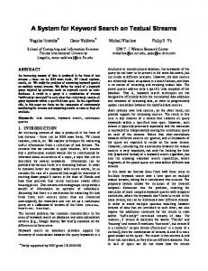
Figure 4: Demonstration of the channel capture effect in Binary Exponential Backoff, as it applies to the experimental setup in [6]. Horizontal axis measures ‘‘locality’’ in the network traffic, expressed as the probability that the identity of the sender of a randomly chosen packet will be the Kth most-recently seen source address on the network, looking backwards in time. Various example configurations from Figures 2−3 are shown, as indicated on each graph.
Using extra measurement data we collected in our simulation model, we have discovered a rather surprising aspect of the Ethernet capture effect. Capture can occur at any time that the network remains congested for some period of time. However, in systems with slow host interfaces, the dynamics of the capture effect consist of the interleaved transmissions by group of hosts, with the group size determined by the maximum transmission rate per host. In Figure 4, we show some new measurements gathered from the actual simulation runs that were used to produce Figures 2−3. These measurements show a generalization of the basic channel capture
9
idea, where one typically counts ‘‘run lengths’’ of consecutive packets with the same source address in the output stream. In this Figure, however, we have adapted the concept of locality from the study of paged virtual memory systems to demonstrate that a group of slow hosts (such as the DEC Titan workstations in [6]) is as effective as a single fast host at monopolizing the channel. To produce this Figure, we maintained a list of host addresses sorted in Most Recently Used (MRU) order. That is, if we look at the list at any time t, then the host currently transmitting (or that transmitted most recently, if the channel is currently idle) will be in position 1, the next most-recently successful host will be in position 2, and so on until the host whose most-recent packet transmission is furthest in the past is at the end of the list. Each time a packet is sent, we increment a counter corresponding to the current position of the sending host in the MRU stack, and apply a cyclic shift to move the sending host to the top of the stack. Thus, the data in this Figure shows the relation between the current MRU stack depth for a host and the probability that it will acquire the network and transmit the next packet. Notice that if there were no capture effect, then all hosts would be equally likely to send the next packet, no matter which ones have been successful recently. Conversely, under complete capture by a single host (i.e., exhaustive service to an overloaded host), we would have probability 1.0 for the lucky host at stack position 1, and 0.0 for all the rest. Looking now at the actual data presented in Figure 4, it is interesting to note how unbalanced these probabilities are — with those hosts that have transmitted recently (and hence are located near the top of the MRU stack) being about 100 times more likely to acquire the channel than the others. Furthermore, the effect of slowing the hosts to include a 100 µsec. reset time merely causes the capturing group to expand from a single host to an alternating pair of hosts (a trio in the case of 64 byte packets), and has virtually no effect on the network acquisition probabilities for the hosts that are deeper in the MRU stack. It is interesting to note that in all 4 system configurations shown, the acquisition probability for hosts deep in the MRU stack is a linear function of the packet length. Thus the data shows that in general, a given host can capture the network for a specific amount of time, rather than for the transmission of a specific number of packets — which is not surprising given that the time constants in BEB (which determine how long the other hosts remain dormant) are independent of the packet size. It is also interesting to compare the locality measure in our data with the predicted run lengths using the simple capacity model that we derived earlier. Consider the measured values of normalized capacity (including 24 bytes of MAC layer overhead per packet in the throughput calculation, as described above) with 64-byte packets and either 8 or 24 active hosts, as reported by Boggs et al. [6]. Using B = 88 bytes and the respective capacity values obtained from [6] into the capacity formula we derived above, we can solve the model to obtain an estimate of the average run length, which is approximately 23 packets using the 8-host capacity value, or 10 packets using the 24 host capacity value. These figures are remarkably close to the results we obtained from our source address locality measurements: if we consider references to the host at MRU stack depths 1 or 2 to be a continuation of the current ‘run’, then we can use the data from Figure 4 to estimate the average run lengths as approximately 25 packets using the 8-host stack reference data, or 15 packets using the 24-host stack reference data. For comparison purposes, Tables 1−2 show the corresponding results for a more traditional measure of the capture effect: the mean, standard deviation, and maximum ‘‘run lengths’’ observed during some of the experiments reported in Figures 2−3. While the magnitude of the run lengths in Table 2 (with Host Reset Time = 0) is impressive, what is perhaps more important is the complete lack of evidence to show that the capture effect is taking place in Table 1 ( with Host Reset Time = 100 µsec.). Furthermore, by comparing the data in any column of Table 2, we can see that the channel holding time by a single host is roughly inversely proportional to the number of active hosts.
10
� ��������������� ��������������������������������������������������������������������������������������������������������������������������������������������������������������������������������������� ������������ ���������������� ������������������ ������������������ ������������Packet ������ ����Sizes ���������������� ������������������ �������������������� ������������������ ����������������� Hosts: � ��������64 128 256 512 768 � ��������������� �������������������� ���������������� ������������������ ������������������ ������������������ �� ����1024 �������������� ������1536 ������������ �� ����2048 �������������� ������3072 ������������ �� ����4000 ����������� 2 1 1 1 1 1 1 1 1 1 1 0 0 0 0 0 0 0 0 0 0 1 1 1 1 1 1 1 1 1 � ��������������� �������������������� ���������������� ������������������ ������������������ �������������������� ������������������ �������������������� ������������������ ������������������ �� ����1����������� 4 1.002 1.002 1.002 1.006 1.009 1.014 1.019 1.031 1.037 1.048 .0593 .0521 .0684 .1569 .1831 .2474 .2861 .4103 .4231 .5026 8 6 6 14 12 14 9 16 14 12 � � � � � � � � � � � � � � � � � � � � � � � � � � � � � � � � � � � � � � � � � � � � � � � � � � � � � � � � � � � � � � � � � � � � � � � � � � � � � � � � � � � � � � � � � � � � � � � � � � � 8 1.008 1.003 1.006 1.017 1.022 1.029 1.051 1.087 1.105 1.139 .1130 .0905 .1121 .2301 .2762 .3060 .4352 0.637 .7103 .8407 10 9 7 10 11 9 12 11 12 14 � � � � � � � � � � � � � � � � � � � � � � � � � � � � � � � � � � � � � � � � � � � � � � � � � � � � � � � � � � � � � � � � � � � � � � � � � � � � � � � � � � � � � � � � � � � � � � � � � � �
16 1.020 1.009 1.017 1.040 1.060 1.076 1.112 1.156 1.204 1.222 .1686 .1353 .1908 .3362 .4462 .5176 .6767 .8153 .9296 1.018 � ���������������������6����������������9������������������9������������������9������������������15������������������12 ��������������������14������������������12 ��������������������11������������������13 �������������
Table 1: Measured run length statistics from the experiments used to create Figure 2, where the Host Reset Time = 100 µsec. Each entry consists of a triple, representing the mean, standard deviation, and maximum run length observed in our re-creation of the experiments from [6]. The data shown provides no indication that the capture effect is present in this system.
� � � � � � � � �� �� � � � � � � � � � � � � � � � � � � � � � � � � � � � � � � � � � � � � � � � � � � � � � � � � � � � � � � � � � � � � � � � � � � � � � � � � � � � � � � � � � � � � � � � � � � � �� ������������� ���������������������������������������� ������������������� ��������Packet ��������� ����Sizes ������������������������������������ ������������������� ��������������������� ��������������� � Hosts: � ��� ������64 � � � 128 256 512 � 768 � 1024 � ������������������ ��� ������������������� ��������������������� ������������������� ������������������� ����������������� ������������������� ������1536 ���������������� ����2048 ���������������� ������3072 ��������������� ����4000 ����������� 1064 800.0 331.8 239.0 190.7 116.1 113.1 72.89 � 57.06 � 2 � � 2358 � � � � � � � � � � � � 1317 � 803.8 � 399.5 � 207.4 � 169.2 � 128.7 � 65.90 � 53.54 � 35.73 � 31.44 � � � 6010 �������������������2169 ����������������� ����875 ��������������� ��679 ��������������� ����492 �������������������219 ����������������� ��249 ����������������� ����166 ����������������� ��141 ������������� ������������������ ��� �������������������� ����2957 � 4 � � 708.9 � 366.0 �� 219.1 �� 106.5 �� 75.86 �� 62.62 �� 42.6 �� 33.22 �� 22.98 �� 18.04 � � � 654.6 � 382.7 � 209.1 � 114.7 � 72.96 � 58.07 � 40.30 � 33.34 � 22.22 � 16.57 � � � 2918 1486 771 441 354 243 158 129 118 72 ������������������ ��� �������������������� ���������������������� �������������������� �������������������� ������������������ �������������������� ���������������������� �������������������� ���������������������� ��������������� � 8 � � 250.8 � 165.2 � 86.12 � 50.78 � 33.45 � 25.22 � 18.79 � 15.39 � 10.23 � 8.31 � � � 324.4 � 208.6 � 106.6 � 59.42 � 37.48 � 28.97 � 19.04 � 15.51 � 10.52 � 7.96 � � � 1637 1258 582 319 194 163 86 72 50 46 ������������������ ��� �������������������� ���������������������� �������������������� �������������������� ������������������ �������������������� ���������������������� �������������������� ���������������������� ��������������� 8.425 6.976 5.038 4.20 � 16 � � 95.51 � 60.95 � 34.19 � 20.03 � 13.53 � 11.34 � � 7.758 � 5.181 � 3.928 � � � 147.2 � 84.16 � 49.29 � 26.95 � 17.66 � 13.56 � 9.54 � � �� � � � � � � � �� �� ��������������������1038 ����������������������493 ������������������382 ������������������192 ����������������122 ��������������������94������������������62������������������59 ��������������������38������������������22 �����������
� � � � � � � � � � � � � � � � � � �
Table 2: Measured run length statistics from the experiments used to create Figure 3, where Host Reset Time = 0 µsec. This time, the run lengths clearly show the significance of the capture effect.
I.c. Lessons from Queueing Theory: Making Users Happy In any system involving a shared resource, one must be careful not to confuse the perceptions of the service provider with those of the users. In the case of a Local Area Network (like Ethernet), the primary concern of the service provider is throughput, i.e., whenever there are packets in the system in need of transmission, the network should be engaged in delivering one of them. The users, on the other hand, are primarily concerned with delay, which consists of both access time (which measures the time that a particular packet spends at the head of its own transmit queue) and waiting time (which measures the time elapsed from the generation of a particular packet until its arrival at the head of the transmit queue). Furthermore, in many applications delay variance (also known as delay jitter ) is at least as important as average delay. It is well known that human users have a strong dislike for unpredictability in receiving the results to an interactive request or the next segment of some continuous media like voice or video. Unpredictable response times also make it difficult to select suitable values for protocol timeouts: even if
11
you knew that the average response time were 1 second, you would still have trouble deciding whether 1.1 seconds, say, was an appropriate timeout value. If each transaction had a deterministic response time of 1 second, then our choice would be fine. However, if 2/11 of the transactions took 0.1 seconds and the remaining 9/11 of the transactions took 1.2 seconds (for an average of 1.0 seconds), then the timeout would expire prematurely more than 80% of the time.3 Both throughput and delay are affected by the ‘‘global scheduling’’ discipline implicitly determined by the MAC layer protocols. That is, following the successful delivery of some packet originating from host X, we wish to find out which packet will be delivered next. The effects of scheduling discipline have been widely studied in the queueing theoretic literature for many decades [8, 17]. For our purposes, the two most important lessons are summarized in a short note by Kingman [16], where he considered a model in which: (i) the scheduling discipline does not know the actual service demands (i.e., packet size, queue length) of each user; (ii) different users (packets) have statistically similar service demands; and (iii) the system is work conserving, which means that the shared resource is always engaged in something useful if there is at least one user waiting for service. Under these conditions, Kingman showed that the average delay is independent of the global scheduling discipline. Furthermore, he also showed that the variance of the delay is minimized if users are selected in first-come−first-served order, and maximized if users are selected in last-come−first-served order. Let us now consider a couple of key ideas from Kingman’s results that help us to see the consequences of various aspects of the Ethernet MAC layer protocols on performance. The most obvious consequence is that the implicit scheduling policy produced by the BEB algorithm is basically ‘‘smallest collision-counter first’’ — which is almost the same as last-come−first-served. Thus, since lastcome−first-served scheduling is the worst thing one can do in terms of maximizing the variability of the response times, Ethernet will have extremely unpredictable response times. There is, however, an even more serious performance consequence to consider, because BEB is not even close to a work conserving scheduling discipline. Consider what happens during a period of congestion. It is not unlikely that some unlucky host(s) will suffer a multiple collisions and ‘‘sleep’’ right through the end of the congested period, waiting for its backoff delay to expire. Obviously, this means that the channel will be sitting idle even though there are packets in the system waiting to be transmitted. However, the implications of this fact can lead to counter-intuitive results in moderately loaded systems, as shown below in Figure 5. Since Ethernet is a shared resource, and each host must compete with the other hosts to acquire exclusive access to that resource before it can deliver any of its packets, it seems logical that performance should improve if a fixed amount of traffic is concentrated among a smaller and smaller number of hosts. For example, if you had file server connected to a heavily loaded network, then you would expect that splitting the network traffic across two network interfaces on the same network would make things worse rather than better, because it would allow the server collide with itself. Surprisingly, as shown in Figure 5, this assumption may not be true under conditions of moderately heavy load (say 50 − 80% utilization) when average delay decreases as the number of hosts increases even if the total load on the system is held fixed. In this Figure, Armyros has used a simulation model to show how the average delay (including access time and waiting time) is affected by the number of active hosts. The system configuration � ��������������������������� 3
Of course it is possible to avoid such a spectacular failure by estimating the variance of the response times along with their mean, and adjusting timeout values accordingly — see [7, sections 12.15 − 12.20]. Nevertheless, this is treating symptoms rather than solving the underlying problem: everyone would be much happier if response times were more predictable, so that tighter timeouts could be used. Indeed, according to the Chebyshev inequality [18, section 3.7], the probability that we are wrong to assume that a transaction has been lost when some given timeout interval expires is proportional to the response time variance.
12
Mean # of frames in a row
Ethernet Response Time . . . . .. . . . .. . . . .. . . . .. . . . .. . . . .. . . . .. . . . .. . . . .. . . . .. . . . .. . . . ..
10
1
s 0.1 e c
0.01
0.001
0.0001 0
0.1 0.2 0.3 0.4 0.5 0.6 0.7 0.8 0.9
100 50 20
. . . . .. . . . .. . . . .. . . . .. . . . .. . . . .. . . . .. . . . .. . . . .. . . . .. . . . .. . . . ..
100
10 5
f r a m 10 e s
1
0.2
0.4
0.6
0.8
2 3 5 10 20
50 100
1
Offered Load
Offered Load
Figure 5: Effect of Number of Active Hosts on Ethernet Response Times (including both waiting time and access time). Solid lines: simulation data by Armyros [5]. Dashed line: approximate analytical formula due to Almes and Lazowska [4], which is based on the simplistic capacity analysis in [21]. Dotted line: predicted capacity using Almes and Lazowska’s formula, which ignores the capture effect.
used to produce this Figure is similar to the one reported by Boggs et al. [6], except that Armyros used a bimodal packet length distribution (with 1/3 ‘‘short’’ 132 byte packets and 2/3 ‘‘long’’ 1096 byte packets, for an average size of 775 bytes) and a symmetric Poisson arrival process at each host. From this Figure, we can see three distinct ‘operating regimes’ at different throughput values. First, when the throughput is less than about 5Mbps, the network is quiet. Here queueing delays are small compared to the transmission time for a packet, and the simple analytical formula developed by Almes and Lazowska [4] is in good agreement with the simulation results, almost by default. The second region covers throughput values between 5Mbps and 8Mbps, where the network is starting to get quite busy. Here the queueing delays blow up suddenly, and we see an unusual inversion of the delay curves where the worst delay performance comes with the fewest active hosts. Note also that the analytical delay formula is grossly optimistic, to the point where the curve does not even exhibit the correct order of magnitude. The final region covers throughput values in excess of 8Mbps, where the network is becoming saturated. Here the delay inversion disappears and the capture effect takes over, allowing the throughput values to exceed the maximum value predicted by the analytical formula by a substantial amount. It is interesting to note the extent to which the capture effect can interfere with the short-term fairness of the protocol: as the network becomes completely saturated, each host in a 2-host system will on average transmit more than 100 frames in a row before allowing the other one to send anything.4 The behaviour of the system when the network is either quiet or saturated is easy to understand. The anomalous behaviour in the middle region occurs because BEB is not even close to a work conserving policy. Under these traffic conditions, the network is still somewhat starved for traffic. However, if � ��������������������������� 4
Notice that in general, these run length numbers are in agreement with those in Table 2 for similar packet sizes (i.e., 768 byte), except for the 2-host system. We attribute this discrepancy to the fact that Armyros’ data is reporting an open system approaching saturation, whereas the data in Table 2 is for a closed system that is at saturation.
13
some host is busy executing a long backoff delay while the channel is idle, that packet and every other packet in the same transmit queue are locked out of the network. As the number of active hosts decreases (for example, by bridging the segment containing a group of clients with another segment containing their main servers), the number of additional packets found in the same transmit queue increases. Thus, the ‘‘suffering’’ caused by a single long backoff delay is shared by many packets. We will also gain some insight from a couple of well-known formulas that give the mean delay in specific queueing systems. In these formulas, we use the notation λ to represent the average customer arrival rate (in customers per unit time), X � and σ 2X to represent the mean and variance of the service time � to represent the utilization of the queue (i.e., distribution (measured in the same units as λ), and ρ ≡ λ X how busy the server is, on a scale of 0 [idle] to 1 [saturated]). The first formula is called the Pollacek-Khinshin (P-K) equation, which gives an exact expression for the mean waiting time in an M/G/1 queue: a system with Poisson arrivals and arbitrary service ��� , is given by the following fordemands for each customer. Here we find that the average waiting time, W mula: 2
� ) λ (σ 2X + X ��� = � ����������������� . W 2 (1 − ρ)
(1)
The second formula is an approximation to the waiting time under heavy load in a G/G/1 queue (which allows both an arbitrary arrival pattern and arbitrary service demands): λ"�"�(σ"�"�2X "�+"�σ"�"�2λ ") " # , !�! = W 2 (1 − ρ)
(2)
where σ 2λ represents the variance of the customer interarrival time distribution. It is interesting to note that Eqs. (1−2) are almost the same, except for one term in the numerator. Thus, the Poisson traffic assumption is really not very important in determining delays in a heavily loaded system, since the approximation in Eq. (2) gets better and better as ρ → 1. The main point of introducing these queueing formulas is to emphasize the importance of service time variability (i.e., σ 2X ) in determining delay, and hence quality of service as perceived by the users, since the ‘‘delay explosion’’ that occurs in a saturated system (i.e., ρ ∼ ∼ 1) is not unexpected. In particular, both equations show that if we keep the utilization of the system fixed, then the mean delay is proportional to the variance of the service times. The added refinement in Eq. (2) merely says that the delay is also proportional to the variance of the customer arrival process (which is fixed at the square of the mean in a Poisson process). I.d. Benchmarking Revisited Let us now take a closer look at the delay implications of the Ethernet measurements reported by Boggs et al. [6]. In section 3.5 of that paper, the authors argued that Ethernet compares favourably with an ideal round-robin system (such as an ideal token ring5), since the relative value of the ‘‘excess delay’’ (i.e., the difference between the measured mean access time in an n-host system and the length of a polling cycle in an ideal n-host round-robin system) is quite small. However, please note that a large Ethernet should enjoy an access delay advantage over a token-passing system under light traffic, since an $ $�$�$�$�$�$�$�$�$�$�$�$�$�$ 5
Note that neither FDDI nor the IEEE 802.5 Token Ring are even close to this ‘‘ideal’’, in which each host is allowed to transmit a single packet for every visit by the idle token. In particular, given an M host network with the right initial conditions the timed-token protocol in FDDI can degenerate into a repeating pattern where each host gets to use all of the asynchronous bandwith during 1 out of every M +1 token rotations and none of the bandwidth during the remaining M out of M +1 token rotations, which results in a very high access delay variance.
14
arriving packet can begin transmission immediately (assuming the channel has been idle for at least an inter-frame gap) instead of waiting for the next visit of the token. Thus, if the network is busy enough for such a comparison to round-robin to make sense, then it should be obvious that waiting times are likely to be much larger than access times, which are beyond the scope of their measurement study. Furthermore, this result merely shows that the average access time is quite reasonable, but shows nothing about its extreme unpredictability. Let us reexamine the data used to compare a heavily loaded Ethernet and an ideal round-robin system in [6], but this time we shall turn our attention to the average waiting time instead of just the average access time. (Remember that their experiment was run on a heavily loaded network, so the 1−ρ term in the denominator of the waiting time expression will ensure that waiting times are much larger than access times.) We shall focus our attention on the transmit queue at a single host, treating the access time for the packet at the head of the transmit queue as its ‘‘service time’’ and use Eq. (1) to estimate the average waiting time experienced by its packets. To be fair to Ethernet, we shall ignore the ‘‘excess delay’’ which would cause ρ to increase and hence bring an already heavily loaded system that much closer to the ‘‘delay explosion’’ at ρ = 1. Thus, the only substantive difference between Ethernet and the ideal round-robin system is in the value of σ 2X . Now in the ideal round-robin system, it should be clear that σ 2X ≡ 0, since each packet transmission will occur according to a fixed schedule. To get the corresponding results for Ethernet, we compare Figures 3-7 and 3-8 from [6] to determine that σX ∼ % ∼ 3.X with 24 hosts (e.g., roughly 65 msec. versus 22 msec. with 1024 byte frames, and 45 msec. versus 12 2 & . With 5 hosts, the ratio is even msec. with 512 byte frames). Thus, σ 2X is about 9 times bigger than X larger because of the convexity of the curves in Figure 3-8: σX ∼ ' and thus σ 2X is about 20 times bigger ∼ 5.X 2 ( . If we now substitute these values into the numerator of Eq. (1), we see that the published data in than X [6] indicates that under heavy load the delay in Ethernet is more than ten times larger than an ideal round-robin system, even if we ignore the ‘‘excess delay’’ effects. I.e. Ethernet as a ‘‘Drop Cable’’ Leading to a BackBone Network or ATM Switch One major trend in the evolution of LANs is that Ethernet may outlive some of its successors (like FDDI) by mutating into a local point-to-point or multi-point drop cable from one’s office to a port on the backbone network — in other words it will become the ‘‘RS-232 cable’’ of the 1990’s. The backbone network may be a higher speed LAN, a ‘‘collapsed backbone’’ multiport bridge or router, or even a Local ATM switch. This evolution allows a substantial increase in the size and/or traffic handling capabilities of a local (inter)network, while preserving the existing investment in Ethernet-compatible ‘‘legacy LAN’’ equipment. Unfortunately, this application brings out the worst in the current Ethernet MAC layer protocols, which were designed for a lightly loaded system with large numbers of slow hosts. For example, consider the extremely low network utilizations reported in the early Ethernet measurement studies, and the following description of the access scheme from [25, section 9]: ‘‘Under normal [emphasis added] load, transmitting stations rarely have to defer and there are few collisions. Thus, the access time for any station attempting to transmit is virtually zero.’’ Similarly, the backoff interval under BEB does not stabilize until it has mushroomed to 1024 slot times — which is far too big for such an application. A power user connected to a backbone switch port by a dedicated Ethernet will expect to be able to load up that channel if necessary. However, because of the very large delay variance caused by BEB, such users are likely to be disappointed with such an arrangement, and therefore with the whole concept
15
of Ethernet connections to a backbone network.6 I.f. Predictable Performance is Worth Something In spite of its dominance of the LAN market over the last decade, the merits and shortcomings of Ethernet remain a subject of intense religious debate. A large part of this controversy is caused by human nature: as with politics, people tend not to trust systems that they don’t understand. Right now, people really don’t know how to evaluate the performance of their Ethernet, and even simple questions like: i. How many hosts can be supported by one network? or ii. How much traffic can be supported by one network? or iii. How many collisions is acceptable? do not have understandable, widely accepted answers — the way we have ‘rules of thumb’ to say that the utilization of a statistical multiplexer should not exceed 80% [27, section 2.4.6]. Thus, rumours spread that Ethernet cannot do X, or that some other technology (say token rings) are better for Y. Furthermore, even the most determined performance analysts will get discouraged when they realize that the delay, say, depends on so many details in addition to the obvious ones of total traffic and number of hosts. In particular, the exact topology (which affects propagation delays) and the exact timing of the traffic generated by each host (which together with topology determines the likelihood of collisions) and the history of channel activity over the last several seconds (which affects the queue lengths and collision counter values at each host) also have a significant influence. When you then pile on the effects of the message generation patterns of the major applications being run at each host, the timeout update algorithms being used by the transport layer protocols, and the capabilities of the network interface, it is tempting to simply give up on performance prediction and claim that Ethernet is some kind of chaotic system. After having spent considerable effort myself in trying to understand Ethernet performance over many years, I have finally reached the following conclusions. First, it was a mistake to call the MAC layer protocol ‘‘CSMA/CD’’, since the real key to understanding its performance lies in capturing the essence of the BEB algorithm. Indeed, in [26] we developed the best currently available formula7 relating throughput, S, to the total transmission attempt rate, G, for unslotted 1-persistent CSMA/CD — but it is almost useless for modelling Ethernet (where we would like to be able to predict the average number of collisions per packet, (G −S)/S, as a function of system load, S) because of the strong influence of BEB on the short-term traffic patterns.
) )�)�)�)�)�)�)�)�)�)�)�)�)�) 6
For certain media, this worst-case MAC-layer performance when Ethernet is used as a point-to-point cable from a workstation to a backbone switch port can be avoided using the proposed ‘‘Full Duplex’’ modification. If the physical layer consists of a pair of unidirectional point-to-point channels (such as twisted pair or an optical fiber), then by disabling the collision detection and loopback circuitry at each end we can treat the network as a pair of independent, collision-free unidirectional channels connecting the transmit circuit on one end to the receive circuit at the other end. However, this solution does not work for any system with more than two devices per collision domain, for systems using coaxial cable, or for 100BaseT4 systems (which use 3 out of 4 wire pairs in parallel to send the data in a single direction). 7 The reader who is familiar with the brief guide to the theoretical studies in [6] may notice that our paper was not included, which is unfortunate because our paper corrected a serious error in the mathematical model of Takagi and Kleinrock [28], which was discussed in section 2.4.6. The correct throughput curve does not have the peculiar double-peaked shape, nor is the maximum throughput limited to 50% even in the zero propagation delay limit — both of which were obviously wrong given the measured throughput data presented in [6].
16
The second conclusion is that it is unlikely that a more accurate analytical model can be found even if we ignore the state of the host and its transmit queue size. Just describing the combined state of the network interfaces for all active hosts leads to a combinatorial explosion: at each end-of-carrier event, we cannot determine what will happen next without knowing both the collision counter value and the remaining time until the current backoff delay (if any) expires for each host [33]. Any progress on finding a suitable model will depend on simplifying the allowable set of states at each end-of-carrier event. The coordinated updates to the backoff counters in the Binary Logarithmic Arbitration Method provide just such a state reduction, and hence the possibility of a performance model that is both tractable and accurate.
II. It Wasn’t Supposed to Work This Way II.a. Binary ‘‘Exponential’’ Backoff is Really a Linear Search for Q Most people don’t understand the intricacies of Ethernet’s Truncated Binary Exponential Backoff (BEB) algorithm. Obviously, the backoff delay intervals selected by a given host increase exponentially with the number of collisions. It is also easy to see that an unlucky host that fails to acquire the Ether after several attempts is doomed to suffer a very large and unpredictable network access delay. However, although no such claim appears in the original Metcalfe and Boggs CACM paper [21], most Ethernet users seem willing to accept this draconian treatment of the oldest packets in the the system, because they believe it allows BEB to defuse ‘‘collision storms’’ exponentially quickly. Unfortunately, as we shall now see, BEB is really just a linear algorithm in terms of its reaction time to a transient overload situation. Thus, it is actually rather slow at adapting to transient overload conditions. For illustrative purposes, let us assume that the cost of each collision is simply one backoff slot time (or 512 bits), so we can determine the running time for the algorithm by counting slot times, rather than getting bogged down in event timing [26] and/or geometric [23] details. Note that each collision includes a 96 bit-time inter-packet space and between 96 and about 570 bit times of activity,8 i.e., the total cost of a collision is roughly 3/8 to 4/3 backoff slot times, so this equal cost assumption will be pessimistic in most cases. Now consider the unhappy situation that would arise if some event triggered a large number of hosts to start transmitting simultaneously. (The possibility of such broadcast storms is well known to network administrators, for example, they can be triggered by configuration errors that cause multiple hosts to attempt to forward broadcasts. They would become routine events if another proposal to ‘‘solve’’ the capture effect were adopted in which the backoff algorithm for all hosts was reset after every successful transmission.) Near the time of such a ‘‘Big Bang’’, it should be obvious that if the number of active hosts is large, none of their early transmission attempts has any hope of succeeding. We can use this fact, together with the simplified initial conditions implied by the ‘‘Big Bang’’ to determine the average time until the first successful packet transmission occurs in such a system. First, we need to determine the probability Pn that a particular host will make another transmission attempt at the nth time step, given that nobody has been successful during the first n −1 steps. Now, recall that under BEB, the starting time for the next attempt will be randomly selected from the next 2min (c, 10) slots, where c counts the number of previous attempts for this packet. Thus, it should be clear that our particular host must select slot 1 for its first attempt, and thereafter it may select slot n for its c +1st attempt only if it selected one of slots n −1, n −2, . . . , n −2min(c, 10) for its cth attempt. Thus, we can * *�*�*�*�*�*�*�*�*�*�*�*�*�* 8
The lower bound comes from the fact that the 32-bit jam cannot begin until a complete 64-bit preamble has been sent; the upper bound comes from a worst-case timing analysis for collisions, described in Appendix A1.3 of the Ethernet Specification [1].
17
determine {Pn } using the equations: Pn =
15
Σ Pn (c)
(3)
c =0
where Pn (c) is the probability that a particular host makes its c +1st attempt in slot n, given that nobody has successfully acquired the channel during the first n −1 steps, and Pn (c) is determined by the following set of recursive equations: P 1 (0) = 1, P 1 (c) = 0
c >0
Pn (0) = Pn −1 (15)
n >1
Pn (c) = Pn (c) =
, ,�P,�k,�(c,�−1) ,�,�, n > 1, c < 10 Σ c c 2 k =max(1, n −2 ) n −1
n −1
(4)
+ +�P+�k+�(c+�−1) +�+�+ n > 1, c ≥ 10 10 10 2 )
Σ k =max(1, n −2
Figure 6 plots the attempt probability in each backoff slot, Pn , as a function of n on a log-log scale over the first 100,000 slots after the ‘‘Big Bang’’ (roughly 5 seconds, which is the ‘‘warmup time’’ in the measurement experiment reported by Boggs et. al, [6]). Two aspects of these (re)transmission rate characteristics of BEB are particularly striking in this Figure. The first is the linearity of 1/Pn over the first 1,000 slots (50 msec.), where the curve is neatly bounded above and below by the simple functions: .- 1- ≤ P ≤ /.2/ n n n (We will come back to the second aspect in the next section.) Note also the distinctive ‘‘saw tooth’’ pattern:9 there is a repeating pattern that includes a local minimum each time the slot number index nears a power of 2 (i.e., slots 2, 4, 8, etc), and a local maximum about half way to the next power of two. This ‘‘modulation’’ of the harmonic function arises in the following way. First, consider the probability density function for the cth attempt, Pn (c). If c is not too small, this random variable is the sum of several independent (but not identically distributed!) other random variables, each of which is one of backoff delays chosen by BEB for this packet. Thus, recognizing that taking logarithms (as we do in the x-axis of Figure 6) greatly reduces the differences between the component random variables, we expect the Central Limit Theorem to come into play, i.e., the sum of independent and similarly distributed random variables should to tend towards a normal distribution. Thus, the pdf for Pn (c), shown as dotted curves in Figure 6, should be ‘‘bell shaped’’, in which case the local maxima in Pn occur in the region where Pn (c) and Pn (c +1) have a significant overlap. In other words, the attempt rate for each host under BEB is just a variation on the harmonic (i.e., 1/n) function, in which a smooth slope has been divided into a series of ‘‘terraces’’ — like farms in a hilly area — according to a pattern where the exponentially increasing width and decreasing elevation change for each new terrace are balanced in a way that preserves the overall harmonic trend.
0 0�0�0�0�0�0�0�0�0�0�0�0�0�0 9
Note that this deviation from a pure harmonic function is more important than simply being unaesthetic, since it means that half the time the probability of having a repeat collision in the next backoff slot will actually be higher than it is now!
18
1.0
. ... . . . . . .. . .. . ... . .. .. . . . . .. . . . .... . . . .. . . . .. . . . .. .. .. . . . .. . . . . . . . . .. . . . .. . . . . . . . .. . . . . . .. .. . . . .. . .. . . . . . . . . . . . . . . . . . . .. .. . . . . . .. .. . . .. . . . . . . . . . . . . . . . . . . .
0.1 Pn
0.01
0.001 1
10
100
1,000
10,000
100,000
Contention Slot Number, n
Figure 6: Network load drops off slowly after the ‘‘Big Bang’’. Solid line indicates the probability, Pn , that a given host will attempt a retransmission in the nth backoff slot, assuming none of its earlier attempts were successful. Dashed lines bounding Pn are the harmonic functions 1/n and 2/n, respectively. Dashed line at lower left is the geometric function 1/2n . ‘‘Arch’’ shaped dotted lines show, from left to right, the component functions Pn (3), . . . , Pn (6).
Given this information about the function Pn , we can calculate the average number of contention slots from the ‘‘Big Bang’’ until the first successful packet transmission. From this data it will be clear that reaction time for BEB to respond to a transient overload condition is a linear function of the number of active hosts, m. We proceed as follows. First, we recognize that, if the number of active hosts is large, then we can treat the actions of each of them independently to arrive at the average number of transmission attempts in each backoff slot. This is precisely the type of situation that can be represented by the binomial distribution, which in the general case may be expressed as: β(M, N, P) ≡ P[M out of N independent trials, each with bias P, comes out positive] 12 N34 P M (1 − P)N −M . = M ∼ β(1,m,Pn ) is the probability that one of the m active hosts acquires In this application, we see that Sn,m ∼ the channel for a successful transmission in the nth backoff slot, given that none of them has been successful in an earlier attempt. (The result is only an approximation because we treat the actions of each host in this slot independently, i.e., we assume that each of them may decide to make another attempt in slot n with probability Pn .) Given this function Sn,m , we can easily calculate Lm , the average number of backoff slots until the first successful transmission occurs, starting from an m-host ‘‘Big Bang’’, using the following formula: 56 78 ∞ n −1 Lm = Σ n Sn,m Π (1 − S j,m ) =
n =1 ∞ 9:
j =1
n
n −1
Σ Σ Sn,m jΠ=1 (1 − S j,m )
n =1 k =1
;
∞
n −1
Σ Σ Sn,m jΠ=1 (1 − S j,m )
k =1 n =k
19
?@
=
∞
Σ
AB
CD Π (1 − S j,m ) ≡
k −1
k =1 j =1
∞
Σ Fk −1 ,
(5)
k =1
where F 0 = 1, and Fk = (1−Sk,m ).Fk −1 for all k >0, represents the probability that all hosts have failed to acquire the network during the first k backoff slot times. Since the function Fk is decreasing at least geometrically fast as k increases, Lm is easy to evaluate despite the infinite summation. Figure 7 shows a plot of Lm as a function of m. Also shown is the sample mean obtained by Monte Carlo simulation, where we have repeated the m-host ‘‘Big Bang’’ experiment until the width of the 95% confidence interval is below 4% of the mean. Notice the excellent agreement between Eq. (5) and the simulation data, especially for m ≥4, which shows that the independence assumption is not very important. Note also that Lm is growing linearly with the number of active of hosts, m, with Lm ∼ ∼ 2/9.m when m >> 1. 500 R e a c t i o n T i m e Lm
200 100 50 20 10 5 2
..
..
..
.
..... . . .. ......... .... . . .. ....... . . . . . ..... . .... .... . .... . . . ... . ... ...... . ..
1 1
2
5
10
20
50
100
200
500
1000
Number of Active Hosts, m
Figure 7: Average time to the first successful transmission after the ‘‘Big Bang’’, starting from m active hosts. Solid line is from Eq. (5), which is approximate because of an independence assumption. Dashed line is the sample mean obtained by Monte Carlo simulation of the exact system. Dotted line is from Eq. (6), which is the equivalent result for the Binary Logarithmic Arbitration Method that will be introduced in section III.
II.b. BEB is Supposed to be Stable for up to 1024 Hosts, but Isn’t Another aspect of Figure 6 worth noting is the convergence to steady-state after the 1000th slot time, as the possibility that the collision counter has ‘‘wrapped around’’ after 16 unsuccessful attempts becomes more significant. In particular, the pattern of damped oscillations has completely decayed to zero in less than 1 second, at which point the steady-state probability that the given host transmits in each backoff slot is approximately10 1/225. This result means that Ethernet using BEB will become bistable if E E�E�E�E�E�E�E�E�E�E�E�E�E�E 10
We can calculate its exact value quite easily using the following argument. The first attempt for a new packet takes exactly 1 slot, the second attempt is equally likely to take 1 or 2 slots, and so on, so the average time until we hit an excessive collision error at the end of the 16th attempt is: 1+2 1+2+3+4 1 + 2 + . . . + 1024 3 5 9 513 1025 13 + 7 ×1024 1 + F F�F�F�F + GHG�G�G�G�G�G�G�G�G . . . + 6 × I�I�I�I�I�I�I�I�I�I�I�I�I�I�I = 1 + JKJ + LKL + MKM + . . . + NKN�N�N + 6 × OKO�O�O�O = P#P�P�P�P�P�P�P�P�P�P . 2 4 1024 2 2 2 2 2 2 Thus, recognizing that a given host makes 16 transmission attempts over such a ‘‘cycle’’, we see that in steady state its contribution to the channel traffic is (13 + 7 ×1024) / 32 = 1/224.4 transmission attempts per slot time. It is also
20
the number of hosts in a single collision domain is significantly larger than 225, and in particular that anything approaching 1024 hosts will be problematic. Thus, if a situation ever arose in such a system where most of the hosts were trying to transmit packets at the same time, there is a chance that the system could enter the ‘‘steady state’’ operating mode, where each host independently cycles around its backoff/retry loop, generating an average of 1 packet every 225 slot times. If the number of hosts is much larger than 225, then almost every attempt will end in another collision and the system will remain in this degraded operating mode for a very long time. Note that bistable behaviour does not necessarily mean that the system, when started from a ‘‘good’’ state (like all hosts quiet), will not work at all. It simply means that eventually it will move from its ‘‘good’’ operating mode to its ‘‘bad’’ one, and possibly back again. The time spent in the ‘‘good’’ operating mode depends on such factors as average load on the system and detailed topology and traffic information, which is beyond the scope of this paper. However, it is important to note that the operation of the system during the ‘‘bad’’ operating mode does not depend on detailed traffic patterns: as long as each host’s transmit queue remains non-empty, its future transmission times are completely determined by the MAC layer protocol. And in particular, since BEB is a discrete time algorithm, synchronizing the transmissions by different hosts to some integer multiple of a slot time beyond end-of-carrier, even topology is of minor importance in an overload situation. Figure 8 illustrates the instability problem with large numbers of hosts. In this Figure, Armyros [5] has used simulation to reproduce the measurement experiments reported by Boggs, et al. [6] on an overloaded Ethernet, so that configurations with many hundreds of hosts could be investigated. What is most striking about this Figure is the dramatic qualitative change in the observed behaviour when we reach hundreds of hosts. (Please note the use of a logarithmic x-axis for most of the graphs.) In particular, most packets suffer an excessive collision error, and the average value of the collision counter for those packets which are successfully transmitted is approaching its maximum value. Note also how the utilization is falling as the number of active hosts increases, especially with short packets. The reversal of the effects of varying the packet size between Ethernet Throughput and Percentage of Dropped Frames can be explained as follows. First, since even the occasional successful transmission of a large packet will contribute significantly to the utilization in bits/sec., utilization is an increasing function of packet size. However, since each of those successful packets occupies the channel for such a long time, many hosts (even those waiting for substantially different backoff timeouts to expire) can enter the deferring state during one of those transmissions. Because of the 1-persistent transmission rule, all of those hosts will collide with each other at the next end-of-carrier event. Thus, the collision rate is also an increasing function of packet size. II.c. But Exponential Backoff Causes Huge Delays for Some Packets, even During Light Load Even though BEB acts globally like a linear search for Q, one must not forget that locally, i.e., from the perspective of an individual host, the backoff delays after each collision are increasing exponentially. As a result, the access time distribution has a very long ‘‘tail’’, i.e., a small fraction of the packets experience delays that are extremely large compared to the mean. As we already discussed in section I.c. in the context of delay variability, the fact that a few packets suffer large delays is important because it interferes with interactive response times and confuses higher-layer protocol adaptive timeout/congestion control algorithms. In other words, if the time constants in higher level protocols are measured in seconds, then even if only one packet from among the thousands transmitted over a second is not delivered in a timely fashion, the user level grade of service may be significantly affected.
Q Q�Q�Q�Q�Q�Q�Q�Q�Q�Q�Q�Q�Q�Q
easy to see that the steady-state solution to Eq. (4) is P 1 (∞) = P 2 (∞) = . . . = P 15 (∞), and hence that we can deduce nothing about the current value of a host’s collision counter from the fact that it chose to transmit now.
21
Ethernet Transmission Delay
4000 .. .. 0.1
s e 0.01 c
0.001
. ..
..
..
.
. ..
..
. ... ..
...
...
..
....
...
.. ....
....
. .. . . . .... .... .. . . .. ... . ... . . ... . .. .. .. .. .. .. .. .. . .. .. . . .. . .. . .. . . .. .. .. .... . ... ... ... ... . .. . .. .. ... . . . .. . . .
Ethernet Throughput 1e+07
3072 . . . . . . 2048 ...
.. . .... ....
1024 . 512
.....
......
256 128 64
b i 8e+06 t s / s e 6e+06 c
. . .. . . . . . . . . . . . . . . .. .. .. .. .. .. .. .. .. . . . . . . . . . 4000 . . . . . . . . . .. .. . . . . . . .. . . . . . . . . . . . . . ... . . . . . . . . . ... . . . . . . .. . . . 3072 .. . . . . . . . . . . . . .. ...... . . . ... . 2048 .. .. . .. .. . ... . . 1024 .. .. .. .. .. .. . .
512
256
128 4e+06
0
100
200
300
400
60
40
20
0
Retransmissions per frame
z
. .+ . . .+ .. + +.+ . .. . . . ××××× .. .256 . . .+ . . . . .+ ×× .. . . . × 4000. . .+ × . . .. ... . . .+ .. × . . .. . . .. × .. .. .. . . .+ . . × . .. .. .. . . . . × . .. . .. . .+ . . . . . .. × . .. .. . .. . . .. .. . . .. . + . .. . . . . . . × . . . .. .. .. .. .. .. .. .. . .. . .. . . . .. . . . × .. .. .. .. .. .. .. . . .. .. . . . . . . . . . . .+ .. .. .. .. . . .. . .. .. .. . . . . . . . . .. .. .. . .. . . .. .. .. ×× .. . . . ×× . . . .. .. . × . . × .. . . .. ×× . . .. .. . . . ×× . . .. .. ×× .... .. . . .. .. × . . . . . . . .. ×× ... .. . . . . 64 .. ×× . . ... . .. × . . . ...... .. ... . . × . . . . . . . × . . . . .. . .. ... . .. . ×. . ×. .. .. . . . . . . ... . . ... .+ . .. .. . . +×. . . . . .+×. .. . .. ×.. .. .. .. . . . . . . . .
{
l m
n
o
p
qr
st u
y vwx
15
1
[ W XYZ V U T R S
`ab \]^_
10
cdefg
. 256 .+ .+ . ..+ .+ × . . . . .+ ××× .¤ . ... . . .+ ××× .£ . .. 4000. . . . . .+. .+××× .. . .¡ .¢ ... .... . . . .+ × . . . . .. . × . . .. . . .+ .. . . . . × . . . .. . . . . . . + . . . ... . .. . .
128 512 × × 1024 +. . . . . .+. 2048 3076 . . . . . . . 64,256,4000
¥
¥
.......
t 10 i m e s
j
R
100
Percentage of Dropped Frames
k
%
10
Number of Hosts
.......
80
1
Number of Hosts
128 512 × × 1024 +. . . . . .+. 2048 3076 . . . . . . . 64,256,4000
{
64
5
hi
0
100
|
1
Number of Hosts
× .. . . . . . . .. . . .. . . × .. . . .. .+ . . . . . . .. .. .. .. . . .. .. .. .. .. .. .. .. × ... .. . . . . .. .. ... . .. .. . . .. + .. .. .. .. . . . . . . . . .. .. .. .. .. . . . .. .. × . . .. . .. . . . × . . . . × . × .. . . .. ×× .. . . .. . . .. ×× . . . . .. .. ×× ... . . . . 64 . × . . . . . .. . . ×× .... . . .. . .. . . ×× . .. × . . ... ... . . × . . . .... .. . . . . . . . × × . . . . .. .. .. . . × . . . . . .. .. . .. . . × . . . . . . . . . . . . . ×. . .. . ..+ . . .. .... . ×. .. .. .. . . . . . . . . . . +×. . . . . .+×. .. .. .. .. . . . . . . .
} ~
10
100
Number of Hosts
Figure 8: Instability in the presence of large numbers of hosts. Results shown were obtained by Armyros [5], who used simulation to extrapolate the measurement experiment of Boggs et al. [6] to systems with hundreds of hosts.
Figure 9 illustrates the effect of this delay variability in a worst-case situation. The data shown is taken from the same simulation experiments used to create Figures 2−3, i.e., a 10-second look at a saturated system in which we vary the packet sizes and the number of active hosts. The data shown represents the maximum observed access time for any host over the 10 second measurement interval in the given experiment, and should be compared with the mean and variance of the access delays shown in the bottom pair of graphs in Figures 1−3 (but note the change of scale from msec. to sec.). It is interesting to note that, unlike the mean and standard deviations, the maximum observed access time does not
22
seem to depend on the number of active hosts.12 Obviously, some other factor must be responsible for these results. We believe it to be the ‘‘wrap around’’ of the collision counter after 16 failed attempts, which causes the given host to suddenly increase the rate at which it attempts to acquire the channel. Using the cycle-time calculation shown in the previous section, we find that the average time until a host declares an excessive collision error is about 51.2 µsec. ×(213 − 15)/2 = 0.21 sec., with the maximum time being twice as large. (In the worst case, deferrals to 16 successful transmissions stretches this at most 25%.) Thus, in most cases, the maximum observed access time seems to represent 2 or 3 complete cycles of the collision counter. 5
M a x D e l a y
5
2
16 8 4
M a x
1
D e l a y
.5
Host Reset Time = 100 µsec 8 Hosts
.2
2 16 1 4 8 2
.5
Host Reset Time = 0 µsec 8 Hosts
.2
.1
.1 64
128
256
512
1024
2048
4000
64
Packet Size
128
256
512
1024
2048
4000
Packet Size
Figure 9: Maximum observed access times (measured in seconds) from some of the experiments used to create Figures 2−3.
Figure 10 shows that these delay variance effects are also present in a lightly loaded production Ethernet environment. To produce this Figure, we inserted a locally designed hardware monitor in series with the AUI cable connecting the departmental netnews server (which is a Sun SPARCstation IPC workstation) to its 10Base5 transceiver. This monitor allows us to record all network events seen on the AUI cable (i.e., start/end of the receive, transmit, and collision signals) with a 1 bit-time resolution, which we can then filter in various ways to record a variety of statistics about network activity. In this experiment, we have selected all packets that experienced at least one collision, and then measured: (i) the cumulative probability distribution function for the access delay, F (x), expressed as the probability that a randomly chosen packet is still in the system x bit times after the start of its first collision); (ii) the conditional probability, G(x), that a randomly chosen host will attempt to retransmit its packet x bit times after the start of its first collision, given that it is still in the system at that moment; and (iii) the conditional probability, S(x), that a randomly chosen retransmission attempt will be successful, given that it occurs x bit times after the start of that packet’s first collision. The results shown are obtained by first accumulating the data into a large number of ‘buckets’, and then merging successive buckets starting at time t using a greedy adaptive algorithm until the number samples in the bucket is proportional to the logarithm of the remaining number of packets in system at time t. Thereafter, each of the above measures is calculated independently for each bucket in the obvious way. Similar results were observed for hosts connected to three other Ethernets, including the Sun SPARCstation 2 workstation in my office, a Silicon Graphics 4D/380 (a major departmental compute server), and an IBM PC compatible desktop computer connected to a mixed Unix/Novell network in the corporate engineering department of a local company. ¦ ¦�¦�¦�¦�¦�¦�¦�¦�¦�¦�¦�¦�¦�¦ The one exception is the 2-host system with Host Reset Time = 100 µsec., in which the protocol dynamics degenerate into round-robin sharing. 12
23
1 P0.1 r 0.01 o b a 0.001 b i 0.0001 l i 1e-05 t y 1e-06
... ... ... ........
... ........ . . . ...
... .. ...... ....... ... . ...... . ..... ... ... ....... . .. .............. . ... ..... ....... ... ... ... ..... ....... . .. .. ........... ...... .......... ..................................................... ... ....... ... .............. .. . .. ........................... .
Pn F (x) G (x)
1e-07 P r0.8 o b 0.6 a b i 0.4 l i t 0.2 y 100
S (x)
1000
10000
100000
1e+06
1e+07
1e+08
Time since first attempt (in bits)
Figure 10: Measured collision retry information for a Sun SPARCstation IPC workstation, which acts as the departmental netnews server. The data shown was derived from monitoring the packet transmission attempts by this host over several weeks. Approximately 94% of the 21.7 million packets transmitted by this host during the measurement period experienced no collisions whatsoever. Notice the large gap in the G (x) function between roughly 1 second and 10 seconds, which we attribute to the time required for the higher layer protocols to respond to an excessiveCollisionError if there are no other packets ready for transmission in the same queue. Note that the upper limit to the time scale represents 10 seconds of elapsed time on a 10 Mbit/sec. network, or 1 second on a 100 Mbit/sec. network.
Several interesting features are evident from these data. The first is the long ‘‘tail’’ of the access delay distribution: even though the network is quite lightly loaded (roughly 2%−10% of the packets experience at least one collision, depending on the time of day), those packets that suffer at least one collision are likely to experience large access delays. To make things more concrete, consider that on a 10 Mbit/sec. Ethernet, the data indicates that 10% of the packets that experienced at least one collision wait for at least 1.5 msec., 1% wait for at least 50 msec., and 0.1% wait for at least 200 msec. between the start of their first collision and the start of their successful transmission. Second, we note the surprisingly good agreement between the predicted harmonic retransmission attempt probability from Figure 5 and the measured data in Figure 10, especially for large values of x
24
where even the ‘‘ripples’’ are in evidence.13 The differences between the predicted and measured curves are caused by deferrals to large packets, which were not considered in the ‘‘Big Bang’’ scenario envisioned in Figure 5. For example, the pattern of a large dip followed by a sudden rise in G (x) that is visible near 12000 bit times is caused by deferrals to some other host transmitting a maximum-length packet. Similarly, if we ignore the spikes due to further deferrals, then the function G (x) is obviously following the function Pn for all x > 50,000 bit times, except for being shifted to the right by the accumulated deferral time. The apparent similarity is improving as x increases because our graph has a logarithmic axis, so the total shift induced by the deferrals, which grows linearly with the number of attempts, becomes proportionally smaller relative to the exponential growth of the accumulated backoff delay. And finally, it is disappointing to see how S (x) for these packets remains quite low, even after many retransmission attempts. That is, even though the probability of success for a first attempt is quite high (i.e., 0.9 − 0.98, depending on the time of day), the probability of success for each retransmission attempt is seldom higher than 0.6, and then drops to about 0.4 after the first millisecond without any significant improvement over time. Note also that the conditional probability of success includes several sharp dropouts — each aligned with one of the major peaks in the retransmission attempt rate curve — which are caused by the ‘‘greedy’’ transmissions-after-deferrals that are characteristic of the behaviour of hosts under 1-persistent CSMA/CD. II.c. Linear Search is a Very Slow Way to Find Q According to [21, section 6], the original motivation for adopting BEB was to approximate the ‘‘optimal’’ 1/Q algorithm,14 in which each of the Q active hosts in the network independently makes a random decision to transmit its next packet in the next slot with probability 1/Q. The idea behind BEB was, therefore, to allow each host to estimate Q in a distributed way, based on the feedback it receives (i.e., success or collision) following each transmission attempt. Unfortunately, as we saw in section II.a., the BEB algorithm is a particularly inefficient estimation scheme for finding Q, because it is really no better than a linear search for Q. The reason for this poor showing is that each host pays attention to only a small fraction of the available information. This is why BEB acts globally like a linear search for Q even though each host is locally reducing its retransmission rate by an exponential amount. In particular, no host ever learns from the (scheduling) ‘‘mistakes’’ of others. Thus, in our ‘‘Big Bang’’ scenario, even if the group of hosts that § §�§�§�§�§�§�§�§�§�§�§�§�§�§ 13
The divergence between Pn and G(x) beyond 3 million bit times coincides with the average time required to complete 16 unsuccessful attempts, which suggests that the given host does not simply go on immediately to the next packet in the transmit queue when an excessiveCollisionError occurs. Indeed, the complete lack of attempts between roughly 1 and 10 seconds suggests that there may be some unusual timeout conditions at work. 14 The 1/Q algorithm is only optimal over the class of memoryless decision rules, and it is easy to apply the principles of group testing [32] and/or conflict resolution algorithms [19] to learn from outcomes of previous decisions to create a more efficient algorithm. For example, consider the average number of time steps until the first successful transmission starting from Q =3. Under the 1/Q algorithm, the probability of success would always be 3.1/31 .(1 − 1/3)2 = 4/9 in every slot, no matter how many unsuccessful slots there are. On the other hand, following a collision at slot k, an algorithm with memory might reserve slot k +1 for all users that did not transmit in slot k. which would lead to a success if and only if one of the three hosts did not participate in the previous collision. In this case, the probability of success in slot k +1 given a collision in slot k can be easily seen to be . 2 .(1 − 1/3)1 ¨�¨�¨�¨�3¨�1/3 ¨�¨�¨�¨�¨�¨�¨�¨�¨�¨�¨�¨�¨�¨ = 6/7 3.1/32 .(1 − 1/3)1 + 1/33 which is almost twice as large as continuing with the 1/Q algorithm. Note also that for large Q, the efficiency of the 1/Q algorithm is no better than slotted Aloha (i.e., 1/e ∼ ∼ 0.368), whereas conflict resolution algorithms can achieve 0.487 under the same conditions.
25
picked the smallest backoff delay for their k +1st attempt experience a collision, the remaining 2k − 1 groups that selected larger backoff delays for their k +1st attempt go ahead with their scheduled transmission attempts anyway, even though those attempts will probably result in collisions too. Thus, even though each host using BEB is going to ‘‘guess’’ the correct estimate for Q within log2 Q ‘‘tries’’, the cost (in elapsed time per algorithmic step) of making each new ‘‘guess’’ is growing exponentially, and so the total running time of the algorithm is linear. Fortunately, global cost of estimating Q can be easily reduced to about log2 Q slot times simply by having each host pay attention to all collisions. That is, whenever a host is waiting for its backoff timer to expire and it sees another collision on the channel, it simply cancels the rest of its backoff interval, increments its collision counter, and proceeds as if it had been an active participant in that collision. It should be clear that under this modification, the global transmission rate function is decreasing exponentially at each successive collision during a contention interval. In other words, even in a worstcase ‘‘Big Bang’’ among Q active users, there will only be about log2 Q collisions in a row until the first success takes place. This binary search strategy is shown as the dashed line in the lower left of Figure 6, and is incorporated into the Binary Logarithmic Arbitration Method that will be introduced below in section III. II.d. The Capture Effect is Accidental During the early days of Ethernet development, it must have seemed inconceivable that a day would come where inexpensive commodity desktop (or even laptop) personal computers would be fast enough to saturate an Ethernet. In any case, there was little reason to worry about the effects of such powerful hosts a decade ago. First, neither contemporary computer system architectures nor their software protocol implementations were incapable of generating traffic that quickly. For example, turnaround times within a query-response message pair were reported to be on the order of 10’s of milliseconds by Shoch and Hupp [25] in 1980, decreasing to about 1 millisecond by the mid 1980’s according to Gusella [13]. Similarly, peak file transfer rates between VAX Unix systems on the order of 0.5 to 1 Mbps were being reported in the early 1980’s [31], and Van Jacobson’s 1988 achievement of 8.9 Mbps between a pair of Sun 3/60 workstations [15] was viewed with a mixture of amazement and skepticism. In addition, network interface designs from that time period paid little attention to supporting high throughput. For example, consider Metcalfe’s recently published list of important network interface design lessons [22]. High on his list was ‘‘The network is seldom the bottleneck.’’ As evidence, he pointed out that disks and operating systems were responsible for limiting the achievable file transfer rates through his early PDP6/10 Arpanet interface to about 20% of its physical line speed. Furthermore, the top priorities at the time were low cost and small size (‘‘Make it fit on one one card.’’ ): sharing the CRC hardware between the sending and receiving sides, using a single on-board packet buffer, and even asking the host to calculate the required backoff delays were all used at one time or another. All of these design tradeoffs stood in the way of high throughput rates by a single host, but nobody cared when the network was so much faster than any of the hosts.
III. A Better Algorithm: Binary Logarithmic Arbitration III.a. Design Goals for the New Algorithm The main purpose for developing the new algorithm is to solve the performance problems described in sections I and II of this paper. More specifically, we have the goals in mind: i. Backwards Compatibility — It would be difficult to change all existing Ethernet devices on a given network to use the new algorithm, and in any case such a massive change could not be done overnight. Therefore backwards compatibility, such that the old and new MAC layer protocols can
26
ii.
iii.
iv. v.
vi.
coexist on the same network, is a top priority. Limited Changes — Even if better algorithms could be designed starting from a ‘‘clean sheet’’, the resulting system must be recognizably an ‘‘Ethernet’’ and not just another incompatible LAN standard. Fairness — The capture effect and non-work conserving properties of Ethernet arise because different hosts can be treated very differently under the current algorithm even though they both participate in the same event (a collision). Improved Response Times — We need to reduce the delays under moderate to heavy load conditions. No Loss in Capacity — This is more of a marketing issue than a technical issue. Nevertheless, the measured capacity of the system according to well-known benchmarking tests should not be sacrificed to meet the other goals. Stability with the Maximum of 1024 Hosts — Although 10Mbps is obviously not fast enough to support anywhere near that number of hosts, a 100Mbps Ethernet may be fast enough, although it is somewhat lacking in geographical coverage. Therefore the MAC layer protocol should not stand in the way.
III.b. Algorithmic Innovations i. It features a logarithmic (instead of linear) time to adapt to transient overloads. ii. The updates to the collision counters at every active host are completely symmetric, so nobody is left ‘‘stranded’’ waiting for a long backoff interval to finish after the congestion is gone. iii. It supports an FDDI-like channel holding time limit to increase channel efficiency in the presence of short packets. After a host has successfully acquired the network during a contention interval, all hosts explicitly concede control of the network to that host until either the holding time limit expires or the host runs out of packets — whichever comes first. This modification allows high throughput values to be achieved even when the average packet length is short, similar to the way that the channel capture effect in BEB helps increase throughput in a congested system. However, unlike the implicit scheduling priority given to the last host to transmit a packet under BEB — which can have serious side effects in terms of delay — our method places a deterministic limit to the channel capture time. (This may be important in environments that use bridging to separate clients and servers when there are lots of short packets, like X-windows.) iv. Our method is an example of a ‘‘limited sensing’’ conflict resolution algorithm, which means that the hosts have no obligation to monitor the channel while their transmit queue is empty. Indeed, the algorithm is specifically designed to allow newly active users to quickly learn the complete system state. Similarly, the disappearance of an active user between its first collision and the successful transmission of its packet does not disrupt the system. However, unlike other limited sensing algorithms (which implement last-come−first-served scheduling), our method implements the processor sharing scheduling discipline, which is more fair and has better delay characteristics. v. Our method supports peaceful coexistence with existing MAC layer devices. Indeed, the addition of some hosts using the new algorithm may even help the performance of the existing hosts. vi. Robustness through automatic, rapid recovery from feedback errors, such as mistaking a successful transmission for a collision or vice versa.
27
III.c. Detailed Description In this section, we present a state-machine based description of the transmit process in each host under BLAM. The description here is obtained by editting the C++ source code and associated comments for the host transmitter process in the SMURF simulator that was used to generate the experimental results shown in this paper. We believe that it is an accurate representation of the MAC level algorithm as it would appear in an Ethernet interface modified to follow the BLAM algorithm. However, a production implementation would require some minor additions to deal with analog signal detection issues. Definitions of Variables and Constants. slotTime standard Ethernet constant, equal to 512 bit times interFrameGap standard Ethernet constant, equal to 96 bit times attemptLimit standard Ethernet constant; recommend increasing from 16 to 20 (See section IV.c.) CCounter the BLAM collision counter variable; replaces standard Ethernet variable attempts. Back BLAM variable containing the most recently generated backoff delay according to the standard Ethernet rule, i.e., a discrete uniform integer multiple of the slotTime over the range 0 . . 2min{CCounter, 10} − 1. BurstStart BLAM variable, used to mark the start of the channel holding time interval for the successful host. BurstLength BLAM constant, holds the maximum time after BurstStart at which the successful host can begin another packet transmission without returning to the arbitration phase. BurstSpace BLAM constant, equal to 192 bit times (i.e., twice interFrameGap ). MaxIdle BLAM constant, equal to 1024 bit times (i.e., twice slotTime ). It is used to control a timeout for decrementing CCounter on the basis of no activity on the channel. CurrentTime the current time. (Any counter running at the channel bit rate will do, since we only care about time differences, rather than absolutes.) Initialization Phase — Newly Active Host Joins the Algorithm 1. Start: This is the initial state, where a host begins the algorithm when it generates its first packet after some period of inactivity. Because of limited sensing, we assume that the host does not know the global state of the algorithm, and initialize the BLAM channel holding timer BurstStart to an undefined value, and CCounter to its initial value of 1. Wait for end-of-carrier (if necessary), then proceed to state doBackoff if we arrived to find no carrier present or we just witnessed the end of a successful transmission. (Note that this means BLAM uses a delayed, instead of immediate, transmission rule for the first attempt. Note, also, that we had a choice of assuming either that some other host is in the midst of a transmission burst, or that a new arbitration period is about to begin. For compatibility with regular Ethernet hosts, we pick the latter, which forces all hosts to begin a new arbitration period.) Otherwise, we must have just witnessed the end of a collision, in which case an arbitration period must be in progress (for which we do not know the correct value of CCounter), so we proceed to state SawCollision. Arbitration Phase — All Active Hosts are Attempting to Acquire the Channel 2. doBackoff: All active hosts are ready to select a new backoff delay following an update to CCounter. The BLAM channel holding timer BurstStart should be undefined, and there should be no carrier present (except, for backwards compatibility with standard Ethernet, we allow hosts involved in a collision to begin their backoff interval at the end of their own jam signal instead of waiting for endof-carrier). Calculate a new backoff delay, Back, using the truncated binary exponential distribution in the usual way, then proceed as follows.
28
3.
4. 5.
6.
7. 8.
9.
If Back=0, then proceed to state Deferring since this host is now committed to a transmission attempt as soon as the interFrameGap has elapsed. Otherwise, if Back ≤ MaxIdle, then set a timeout for CurrentTime + Back and wait for the next event, which may be: (i) start-of-carrier, in which case we go to state OtherBusy, or (ii) timeout expired, in which case we go to state Deferring. Finally, if Back > MaxIdle, then set a timeout for CurrentTime + MaxIdle and wait for the next event, which may be: (i) start-of-carrier, in which case we go to state OtherBusy, or (ii) timeout expired, in which case we go to state TooQuiet. TooQuiet: We assume that an idle period longer than MaxIdle means that our estimated value of Q is gotten too large. Reset CCounter to max {CCounter −1, 1} and return to state doBackoff. (Note: A more complex state machine with slightly better randomizing properties would update the backoff interval after an change in CCounter via Back = floor(Back / 2) − slotTime, where the floor and division can both be done using a shift, instead of recreating it from scratch in state doBackoff. This change has the advantage of ensuring that any host that chose Back = MaxIdle would not have to change its scheduled transmission time.) Deferring: The host is now committed to a transmission attempt. Follow the standard Ethernet deference rule to ensure a proper interFrameGap and proceed to state Xmit. Xmit: This host begins transmitting a packet. Assign BurstStart = CurrentTime, in case this turns out to be a success and wait for the next event. If a collision is detected, proceed to state XAbort. Otherwise, proceed to state XDone when the transmission is finished. XAbort: This host detected a collision during its transmission attempt. Assign BurstStart = undefined, CCounter = CCounter + 1, and wait until the complete preamble has been transmitted (if necessary). Start transmitting a JAM pattern and proceed to state JDone. JDone: If CCounter=attemptLimit, then report an excessiveCollisionError and assign CCounter = 1. Wait for transmission of the JAM pattern to finish and proceed to state doBackoff. OtherBusy: One (or more) other hosts transmitted before we did. Assign BurstStart = CurrentTime in case it turns out to be a successful transmission, and wait for end-of-carrier. If we just witnessed a collision, then the arbitration phase is continuing so proceed to state SawCollision. Otherwise, the other host has acquired the network and we proceed to state SawSuccess. SawCollision: We just witnessed a collision involving other hosts. Assign BurstStart = undefined, since no host managed to acquire the channel. Also, since all updates to CCounter are symmetric under BLAM, assign CCounter = CCounter + 1 even though we did not participate in the collision. If CCounter=attemptLimit, then report an excessiveCollisionError and assign CCounter = 1. Proceed to state doBackoff.
Another Host has Acquired the Network for a Transmission Burst 10. SawSuccess: We just witnessed the end of a successful transmission by some other host, so all active hosts should reset their local copy of CCounter to 1 in preparation for the eventual start of the next arbitration period. In the mean time, we must decide whether or not to concede control of the network to the successful host. If currentTime − BurstStart < BurstLength − interFrameGap , then under BLAM the successful host must be permitted to send another packet without interference. In that case, set a timeout for CurrentTime + BurstSpace and wait for the next event, which may be: (i) start-of-carrier, in which case we proceed to state MoreBusy, or (ii) timeout expired, in which case we proceed to state OtherDone. Otherwise, the channel holding time condition must have failed: assign BurstStart = undefined and
29
proceed to state doBackoff. 11. OtherDone: The successful host ran out of packets before its channel holding timer expired. Assign BurstStart = undefined and proceed to state doBackoff. 12. MoreBusy: The successful host is continuing to send packets in a burst. Wait until end-of-carrier. If we just witnessed another successful transmission (the normal case), then proceed to state SawSuccess. Otherwise, we witnessed a collision, so we proceed to state SawCollision. (Collision are caused by hosts that are either newly active, and do not know the state of the algorithm, or are using the standard Ethernet algorithm, and do not obey BLAM.) This Host has Acquired the Network for a Transmission Burst 13. XDone: This host has completed a successful packet transmission. Thus, it is entitled to continue its current burst until its burst length timer runs out, if it can begin transmitting another packet before the other hosts time out and enter state OtherDone. More precisely, if: (i) this host cannot begin its next packet transmission before the channel holding timer expires, i.e., currentTime − BurstStart ≥ BurstLength − max{interFrameGap, Host Reset Time}, or (ii) the interpacket spacing will be too large to prevent the other hosts from triggering its inactivity timer, i.e., BurstSpace − Host Reset Time ≤ interFrameGap / 2, or (iii) the host’s transmit queue is empty, then its transmission burst is over: assign BurstStart = undefined and proceed to state Start. Otherwise, this host can continue its transmission burst: wait for the host interface to be reset (if necessary) and proceed to state XMore, if start-of-carrier is not detected in the mean time, or to state XRobbed, otherwise. 14. XMore: This host expects to transmit another packet without interference from anyone else (except for newly active hosts, and those using the standard Ethernet algorithm). Follow the standard Ethernet deference rule to ensure a proper interFrameGap, then start transmitting the next packet, and wait for the next event. If a collision is detected, proceed to state XAbort. Otherwise, proceed to state XDone when the transmission is finished. 15. XRobbed: This host had its transmission burst cut short by a collision. Assign BurstStart = undefined, and proceed to state Start.
IV. Performance Comparison IV.a. Logarithmic versus Linear Reaction Time Recall that in Section II.a, we showed that BEB is a linear search algorithm, in terms of both the rate at which the estimated value of Q increases (Figure 6) and also the average reaction time to a transient overload from the ‘‘Big Bang’’ to the first successful packet (Figure 7). We now show that BLAM has a fundamental advantage over BEB in terms of its time complexity under these operating conditions. First, BLAM is essentially a linear search for the logarithm of Q (i.e, a logarithmic search for Q). To see this, consider what happens when the first collision is encountered following the most recent update to the collision counter. In this case, all hosts: (i) cancel the remainder of their current backoff delay (if any); (ii) increment their collision counter (thereby doubling the backoff interval, if CCounter was below 10); and (iii) initiate a new backoff delay uniformly distributed over the new backoff interval — whether or not they participated in that collision. Thus, like BEB we search for Q using exponentially increasing increments. However, unlike BEB, the ‘cost’ per search step is always one backoff slot time rather than an exponentially increasing number of backoff slot times. Second, the average time from the ‘‘Big Bang’’ until the first successful packet transmission is also proportional to the logarithm of Q. Indeed, this O(log2 Q) time complexity means that BLAM is fast enough to allow us the luxury of globally resetting the collision counters after a successful packet
30
transmission to improve fairness. To establish this result, we must find the average number of algorithmic ‘steps’ (i.e., time, in units of a backoff slot time) from the moment that one successful packet transmission triggers all active hosts to reset their collision counter until the start of the next packet transmission. We do this by solving a system of equations defining the average running time of the algorithm as a function of Q. Following the notation from section II.a., we define Lm (C, I) as the average number of backoff slots from now until the first successful transmission occurs in an m-host system, given that all active hosts currently have a collision counter value of C, 1 ≤ C > 1, when one is careful to include in B the 24 bytes of overhead described in [6]. Indeed, all the entries in each column are quite close to the limiting value multiplied by 1/(1−1/M) = M /(M −1), which is the average run length under processor sharing.
33
´ ��������´ ´ �������������������������������������������������������������������������������������������� ´ ´´ ®�®�®�®�®�´®�®�®�®�®�®�®�®�®�®�´ ®�®�®�®�®�®�®�®�´®�®�®�®�®�®�®�®�®�®�´ ®�®�®�®�®�Packet ®�®�®�®�´®�®�Sizes ®�®�®�®�®�®�®�®�´ ®�®�®�®�®�®�®�®�®�´®�®�®�®�®�®�®�®�®�®�´ ®�®�®�®�®�®�®�®�®�´®�®�®�®�®�®�®�®�® ´ Hosts: ´ ®´ ®�®�®�®�64 ´ ´ ´ 128 256 ´ 512 768 ´¯ �¯�¯�¯�¯�¯�¯�¯�´ ´ ¯�¯�¯�¯�¯�¯�¯�¯�¯�¯�´ ¯�¯�¯�¯�¯�¯�¯�¯�¯�´ ¯�¯�¯�¯�¯�¯�¯�¯�¯�´ ¯�¯�¯�¯�¯�¯�¯�¯�¯�´ ¯�¯�¯�¯�¯�¯�¯�¯�¯�´¯�´ ¯�¯�1024 ¯�¯�¯�¯�¯�¯�¯�´´ ¯�¯�¯�1536 ¯�¯�¯�¯�¯�¯�´¯�´ ¯�¯�2048 ¯�¯�¯�¯�¯�¯�¯�´´ ¯�¯�¯�3072 ¯�¯�¯�¯�¯�¯�´¯�´ ¯�¯�4000 ¯�¯�¯�¯�¯�¯ 2 37.30 20.71 12.38 6.234 4.170 4.217 2.105 2.09 2.090 2.043 ´ ´´ ´ ´ ´ 26.54 ´´ 14.99 ´´ 9.180 ´´ 4.427 ´´ 3.064 ´´ 3.064 ´´ 1.484 ´´ 1.543 ´´ 1.553 ´´ 1.399 ´ ´´ °�°�°�°�°�°�°�´°�´ °�151 °�°�°�°�°�°�°�°�´´ °�°�84°�°�°�°�°�°�´°�´ °�39 °�°�°�°�°�°�°�°�´´ °�°�32°�°�°�°�°�°�°�´°�´ °�26 °�°�°�°�°�°�°�°�´´ °�°�12°�°�°�°�°�°�°�´°�´ °�13 °�°�°�°�°�°�°�°�´´ °�°�14°�°�°�°�°�°�°�´°�´ °�11 °�°�°�°�°�°�° ´° �°�°�°�°�°�°�°�´ ´ °�°�342 4 23.98 13.18 7.964 4.020 2.670 2.717 1.349 1.375 1.356 1.349 ´ ´´ ´ ´ ´ 13.14 ´´ 6.965 ´´ 4.304 ´´ 2.088 ´´ 1.371 ´´ 1.425 ´´ .6946 ´´ .7055 ´´ .6956 ´´ 0.669 ´ ´ ´ 126 70 48 24 14 13 7 6 10 6 ´± �±�±�±�±�±�±�±�´ ´ ±�±�±�±�±�±�±�±�±�´±�´ ±�±�±�±�±�±�±�±�±�´´ ±�±�±�±�±�±�±�±�´±�´ ±�±�±�±�±�±�±�±�±�´´ ±�±�±�±�±�±�±�±�±�´±�´ ±�±�±�±�±�±�±�±�±�´´ ±�±�±�±�±�±�±�±�±�´±�´ ±�±�±�±�±�±�±�±�±�´´ ±�±�±�±�±�±�±�±�±�´±�´ ±�±�±�±�±�±�±�± 8 19.74 10.97 6.602 3.313 2.236 2.229 1.143 1.142 1.150 1.145 ´ ´´ ´ ´ ´ 8.078 ´´ 4.486 ´´ 2.624 ´´ 1.293 ´´ .8218 ´´ .8166 ´´ .4106 ´´ 0.408 ´´ .4222 ´´ .4100 ´ ´ ´ 108 50 31 18 10 10 6 4 4 5 ´² �²�²�²�²�²�²�²�´ ´ ²�²�²�²�²�²�²�²�²�´²�´ ²�²�²�²�²�²�²�²�²�´´ ²�²�²�²�²�²�²�²�´²�´ ²�²�²�²�²�²�²�²�²�´´ ²�²�²�²�²�²�²�²�²�´²�´ ²�²�²�²�²�²�²�²�²�´´ ²�²�²�²�²�²�²�²�²�´²�´ ²�²�²�²�²�²�²�²�²�´´ ²�²�²�²�²�²�²�²�²�´²�´ ²�²�²�²�²�²�²�² 16 18.36 10.19 6.134 3.088 2.082 2.076 1.062 1.061 1.063 1.056 ´ ´´ ´ ´ ´ 5.667 ´´ 3.166 ´´ 1.899 ´´ .8388 ´´ .5468 ´´ .5525 ´´ 0.258 ´´ 0.248 ´´ .2641 ´´ .2467 ´ ´´ ´ ´ ´ ´ ´ ´ ´ ´ ´ ³ �³�³�³�³�³�³�³�³�³�³�72³�³�³�³�³�³�³�³�³�40 ³�³�³�³�³�³�³�³�³�24³�³�³�³�³�³�³�³�12 ³�³�³�³�³�³�³�³�³�³�³�8³�³�³�³�³�³�³�³�³�8³�³�³�³�³�³�³�³�³�³�4³�³�³�³�³�³�³�³�³�3³�³�³�³�³�³�³�³�³�³�4³�³�³�³�³�³�³�³�³�4³�³�³�³�³�³
´ ´ ´ ´ ´ ´ ´ ´ ´ ´ ´ ´ ´ ´ ´ ´ ´ ´ ´
Table 3: Measured run length statistics from the experiments used to create Figure 11, which are identical to those shown in Table 2, except for replacing BEB by BLAM.
Figure 13 shows how introducing BLAM reduces the worst-case access delays in an overloaded system. Just as Figure 9 reports the worst-case access delays under BEB for some of the experiments used to create Figure 3, we have in Figure 13 reported the equivalent worst-case access delays under BLAM that were obtained from the corresponding set of experiments used to create Figure 11. Figure 13 shows that, in general, worst-case access delays are insensitive to the packet size. This is to be expected under this type of overload situation, since all hosts will simply keep transmitting until the channel holding timer expires. The only exception to this is for the (illegal) 3072 and 4000 byte packets, where a single packet transmission lasts for significantly longer than a channel holding time. The Figure also shows that the worst-case access delays are growing linearly with the number of active hosts. This is expected, since BLAM tries to ensure fairness in the processor sharing sense, such that the time until any given host from among M active hosts acquires the channel will be geometrically distributed (in multiples of the channel holding time) with parameter 1/M. .5 16
.2
8
.1
4
D e .05 l a y .02
2
M a x
.01 64
128
256
512
1024
2048
4000
Packet Size
Figure 13: Maximum observed access times (measured in seconds) from some of the experiments used to create Figure 11. These experiments are identical to the ones reported in Figure 9, except for replacing BEB by BLAM in all hosts, but please note the change in scale for the y-axis.
Figures 14−16 show the comparative throughput−delay characteristics of BEB (indicated by dashed lines) and BLAM (indicated by solid lines) for a variety system configurations. In all cases, the numbers and placement of the stations follows the experimental setup of Boggs et al. [6], but in this case
34
we assume a symmetric Poisson traffic source at each host. Each Figure reports on the results for a fixed packet size, where both the total utilization and the number of hosts is varied. Notice that in all cases, the results for BLAM are significantly better than for BEB — especially in the middle region where the network is becoming moderately busy. In particular, the average queueing delay for BEB is often 10 or 100 times larger than for BLAM in this region, which is exactly what we expect to see, based on Eqs. (1−2), because of the substantially lower access time standard deviation under BLAM. IV.c. Excessive Collision Errors Really Mean Something is Wrong Recall that under BEB, the MAC layer state machine reports an excessiveCollisionError whenever a given packet is experiences 16 collisions in a row. Unfortunately, this ‘‘error’’ is not an indication that something is wrong with the network. For example, Figure 10 shows that the probability of a repeat collision on a retransmission attempt does not decay with the number of retries, even on a relatively quiet network. Thus, since an excessiveCollisionError is a normal (albeit rare) event on even modestly active networks, their occurrence is not useful to higher layer network management functions in trying to diagnose failure conditions.15 Under BLAM, on the other hand, the update policy for the collision counter has been changed significantly, such that every host resets its collision counter after every successful packet transmission on the network. While we made this change to promote fairness, it has the added benefit of turning the excessiveCollisionError into a useful network diagnostic signal. We can show this in two different ways. First, in Figure 17, we show the maximum observed collision counter values in many of the simulation experiments we have described earlier in this paper. The left column of graphs in the Figure show the maximum observed collision counter values over 1000 seconds of simulated time as a function of normalized throughput for an open system with Poisson arrivals and various combinations of packet lengths and numbers of active hosts. The data are obtained from the simulation experiments we used to create Figures 14−16. The right column of graphs uses data from the experiments we used to create Figures 2, 3 and 11, which follow the methodology described in [6]. They show the maximum observed collision counter values over a 10 second measurement period as a function of the number of active hosts in a saturated system, for the same set of packet lengths. Using Figure 17, we can see that in general, the behaviour of collision counter is qualitatively very different between BEB and BLAM. For example, in the the maximum observed collision counter values in the saturated systems are 10 times larger using BEB instead of BLAM, but there is little sensitivity to either the packet sizes or numbers of active hosts.16 Similarly, for the open systems, the maximum collision counter value is both larger and growing much faster under BEB than BLAM.
µ µ�µ�µ�µ�µ�µ�µ�µ�µ�µ�µ�µ�µ�µ 15
For example, in the original repeater specification [1], the network partitioning algorithm is triggered if the number of consecutive collisions exceeds a threshold of at least 30. This same collision count limit was also included in the draft of the 100BaseT repeater that was distributed at the March 1994 802 Plenary meeting, although there was some discussion about raising the threshold to at least 50 consecutive collisions. 16 Of course, using a Host Reset Time of 100 µsec causes an anomaly in the case of 2 hosts because collisions are impossible after the first successful transmission occurs. Note also that increasing the Host Reset Time tends to make things worse for BEB, which we can attribute to the fact that channel capture involves a group of hosts — all of which have (very) small collision counters, and must be ‘‘beaten’’ by the given host before it can acquire the channel.
35
100
50
20 A c c e s s D e l a y
100
. . . . . . . . . . . . . . . . . . . . . . . . . . . . . . . . . . . . . . . . . . . . . . . . . . . .
50
8 A c c e s s
16
10
16 8
5
8 4
D e l a y
4
2
2 2
1
8 5 4 2 2
0.2
0.2
0.1
16 2
10
0.5
. . . . . . . . . . . . . . . . . . . . . . .
4
20
1 D e v 0.5
. . . . . . . . . . . . . . . . . . . .
16
0.1 0
0.2
0.4
0.6
0.8
1
0
0.2
Utilization (Without Overhead)
16 8 4 2
100
Q u 10 e u e i n 1 g
16 8 4 2
D e l 0.1 a y
0.01
0.001 0.2
0.4
0.6
0.6
0.8
1
Utilization (Without Overhead)
1000
0
0.4
. . . . . . . . . . . . . . . . . . . . . . . . . . . . . . . . . . . . . . . . . . . . . . . . . . . . . . . . . . . . . . . . . .
0.8
1000
. . . . . . . . . . . . . . . . . . . . . . . . . . . . . . . . . . . . . . . . . . . . . . . . . . . . . . . . . . . . . . . . . .
16 8 4
100
2 16 8 4 2
Q u 10 e u e S t d
1
D e 0.1 v
0.01
0.001 1
0
Utilization (Without Overhead)
0.2
0.4
0.6
0.8
. . . . . . . . . . . . . . . . . . . . . . . . . . . . . . . . . . . . . . . . . . . . . . . . . . . . . . . . . . . . . . . . . .
1
Utilization (Without Overhead)
Figure 14: Comparison of the Mean and Standard Deviation of the Access Time and Queueing Delay between the Standard Ethernent and the Binary Logarithmic Arbitration Method, assuming 1024 byte packets, symmetric Poisson arrivals, and various numbers of hosts. Network topology follows the experimental setup in [6]. Dashed lines represent a system with only Standard Ethernet hosts, while solid lines represent the same system using BLAM.
36
50
20
10 A c c e s s
5
50
. . . . . . . . . . . . . . . . . . . . . . . . . . . . . . . . . . . . . . . . . . . . . . . . . . . . . .
16 20
A c c e s s
16
2
8 8
D 1 e l a 0.5 y
D e l a y
4 4 2 2
0.2 .
. . . . . .
. . .
. .
. . .
. . . . . . . . . . . . . . . . . . .
. . .
. .
. . .
. .
D e v
8 16 4
10
2 8
5
2
4
1 2 0.5
0.2
0.1
0.1
0.05
0.05 0
0.2
0.4
0.6
0.8
1
0
0.2
Utilization (Without Overhead)
0.4
0.6
0.8
16 16 8 4 100
2 8
Q u 10 e u e i n 1 g
4 2
D e l 0.1 a y
0.01
0.001 0.2
0.4
0.6
1
Utilization (Without Overhead)
1000
0
. . . . . . . . . . . . . . . . . . . . . . . . . . . . . . . . . . . . . . . . . . . . . . . . . . . . . . . . . . . . . . . . . .
0.8
16 1000
. . . . . . . . . . . . . . . . . . . . . . . . . . . . . . . . . . . . . . . . . . . . . . . . . . . . . . . . . . . . . . . . . .
. .
16 .. 8 4
100
2 8 Q u 10 e u e S t d
4 2
1
D e 0.1 v
0.01
0.001 1
0
Utilization (Without Overhead)
0.2
0.4
0.6
Utilization (Without Overhead)
Figure 15: Repeat of Figure 14 using 256 byte packets.
37
0.8
. . . . . . . . . . . . . . . . . . . . . . . . . . . . . . . . . . . . . . . . . . . . . . . . . . . . . . . . . . . . . .
1
20
10
5
A c c e s s
2
20
. . . . . . . . . . . . . . . . . . . . . . . . . . . . . . . . . . . . . . . . . . . . . . . . . . . . . . . . . . . . . . . . . . . . . . . . . . . . . . . . . . . . . . . . . . . . . .
16 10
4 16 5 A c c e s s
16
1
0.1
2 8
2
1
4
D e 0.5 l a y
8 8
0.5 D e l a 0.2 y
8
4 4
2
0.2
D e v 0.1
2 2
0.05
0.05
0.02
0.02 0
0.2
0.4
0.6
0.8
1
0
0.2
Utilization (Without Overhead)
1000
16 8 4
100
2 16 Q u 10 e u e i n 1 g
8
4
2
D e l 0.1 a y
0.01
0.001 0
0.2
0.4
0.6
0.4
. . . . . . . . . . . . . . . . . . . . . . . . . . . . . . . . . . . . . . . . . . . . . . . . . . . . . . . . . . . . . . . . . .
0.6
0.8
1
0.8
1
Utilization (Without Overhead)
1000
. . . . . . . . . . . . . . . . . . . . . . . . . . . . . . . . . . . . . . . . . . . . . . . . . . . . . . . . . . . . . . . . . .
16 8 4 16 2
100
Q u 10 e u e S t d
8
4
1
2
D e 0.1 v
0.01
0.001 0.8
1
0
Utilization (Without Overhead)
0.2
0.4
0.6
Utilization (Without Overhead)
Figure 16: Repeat of Figure 14 using 64 byte packets.
38
. . . . . . . . . . . . . . . . . . . . . . . . . . . . . . . . . . . . . . . . . . . . . . . . . . . . . . . . . . . . . . . . . .
M a 100 x
M a 100 x 16 8 4 2
C C o 10 u n t e r1
C C o 10 u n t e r1
16 8 4 2
0.2
0.4
0.6
. .. . . . . . . . . . . . . . .. .. . . . . . .......... . ... .. . . . .. . . .. . . . . . . . . . . . . . . . . . . . . . . . . . .
0.8
0
1
5
10
Normalized Throughput M a 100 x
M a 100 x
0.4
0.6
0.8
.. . . . . . . . . . . . . . . . . . . . . . . . . . . . . . .
C C o 10 u n t e r1
16 8 4 2
0.2
0
1
.. . ... .
M a 100 x
0.4
0.6
0.8
. ..
..
. . . . . ... .. . . . . . . .. .... .. . . . . .. . . . . . . .
5
10
15
20
. . .. . . ... .. .. . . .. . . . . . . . . . . . . . . . . . . . . . . . . . . . . . . . .. .. . . . . . . . . . . . . . . . . . . . . . . . . . . . . .
C C o 10 u n t e r1
16 8 4 2
0.2
29
256 256
25
29
Number of Hosts
16 8 4 2
C C o 10 u n t e r1
25
256
Normalized Throughput M a 100 x
20
64
Number of Hosts
16 8 4 2
C C o 10 u n t e r1
15
64 64
0
1
Normalized Throughput
5
10
15
20
1024 1024
1024
25
29
Number of Hosts
Figure 17: The maximum observed collision counter values from several of the simulation experiments used to create Figures 14−16 (left column) and Figures 2, 3 and 11 (right column). In each case, BEB with Host Reset Time 100 µsec. is shown as a dotted line, BEB with Host Reset Time 0 is shown as a solid line, and BLAM is shown as a dashed line.
Second, we can use analytical techniques to determine the distribution of collision counter values at packet departure instants under BLAM, as a function of the number of active hosts. That is, we wish to find the sequence FCC (k), which for graphical clarity we define as the probability that the collision
39
counter in a departing packet is greater than or equal to k. For any given value of k, FCC (k) can be found from a transient analysis of the embedded Markov chain defined at those times when the value of the collision counter is updated, i.e., new packet (initialized to 1), collision (incremented by 1), and second consecutive idle (decremented by 1). That is, we assume that both CCounter = k and a successful transmission are ‘absorbing states’ for the Markov chain, and calculate the probability that the system, when started from CCounter = 1, will be ‘absorbed’ by state k instead of the success state. Since the evolution of the collision counter is Markovian (i.e., its next value depends only on the current value and the channel outcome during the next backoff slot time), we can solve for FCC (k) using the following system of equations. Let f j be the probability that the system will eventually enter the ‘absorbing’ state (i.e., CCounter = k), given that CCounter = j in the current state. Given the definition of BLAM, it should be clear that: (i) CCounter changes only in unit increments; (ii) each collision triggers an increase; and (iii) two consecutive idles trigger a decrease. Thus, by comparing the absorption probabilities now and one time step in the future, we can establish the following system of balance equations: ¶· P 1,2 . f 2 j =1 ¸· f j = P j, j −1 . f j −1 + P j, j +1 . f j +1 1 < j < k (7) ¹ 1 j =k , where the transition probabilities, Pi, j are given by P j, j −1 = P[ two consecutive idle slots starting from CCounter = j | M active hosts ] = β(0, M, 1/B).β(0, M, 1/(B −1)) P j, j +1 = P[ collision, or idle followed by collision, starting from CCounter = j | M active hosts ] = 1 − P j, j −1 − β(1, M, 1/B) − β(0, M, 1/B).β(1, M, 1/(B −1)) , and B = 2min{j, 10} is the current length of the backoff interval. Rearranging terms in Eq. (7), we obtain: f 2 = f 1 / P 1,2 f j +1 = (f j − f j −1 .P j, j −1 ) / P j, j +1 0 < j < k ,
(8)
subject to the boundary condition that fk = 1. Notice that we can use Eq. (8) to calculate the entire sequence {f j } to within a normalization constant in one pass, by assuming an arbitrary value for f 0 and then using the boundary condition for fk to normalize the results. Thus, since FCC (k) ≡ f 1 , we can quickly derive the entire distribution function by finding any non-normalized solution, ˆf j , to Eq. (8) and using FCC (k) ≡ ˆf 1 / ˆfk . In particular, if we apply the (non-normalized) boundary condition ˆf 1 = 1, then we see immediately that: 1 FCC (k) = º �º , ˆfk where ˆf 1 = 1 and {fˆj } are obtained, recursively, from Eq. (8).
40
(9)
1 10−2 P r 10−4 o b −6 10 a b −8 i 10 l i 10−10 t y −12 10
. .. ... .. .. . .. .. ..+ +. . .. .. ...+ +. . . . .+... .. ... ... ...+ +... ... ...... ....+ +... .. ... ... ...+ +... .. ... ... ...+ +... .. .. ... ...+ +... .. .. .. ..+.. . . . . . +.. .. .. . ..+ .. + .. + .. + .. + . . +. . +. . . . .+. . . +. . . + . . . . +. . . .+. . .+. . .+. . .+. . .+. . .+. . . .+. . . .+. . .+. . . . .+. . . .. ... . . .. .. .. .. .. .. .. .. +. . . . . .. .. .. .. .. .. .. .. .. +. . +. . . . . . . . . . . . . . +.. +. +. +. +. +. +. +. . +. . . . . .. . + . . . . . . . +. . . . . .. .. . . .. .. . . .. .. .. .. . .. +. . . . . .. .. . .. . + .. . . . +. . . . . . + . . .. . . . . .. . .. . + .. .. + +.. +... +... +... +... +... +. . . .. . . .. . . . . . . . + . . . . . . . +. . . .. .. . . . . . . .. . . . . .. . . .. . . .. . . +. . . . .. . . . + . . . . . . + . .. . .. . . . . . . . +. + .. + + .. . . +. . . . . + . . . . . +.. .. .. . .. . . . . . . . . . . . +. . . .. + . . . . . . . .. . + .. . . . . . . . . .. . . . . . +. . . . . . . . .. . . .. . . . . . + . . . . + . . . .. . . . . . . . .. . . .. . . . . . +. . .. . +.. +... +.. +... . . +. . . . . +.. . . . . . . . . . . . .. . . . . . . . . . . .. . . . . . . + . . . +. . . . . . . . . .. . . . . . . . . . . . .. . . . . . + . . . . . . .. . . . . . . . . .. +.. . . + +. . . . . . +. . . . . .. . + . . . . .. . +.. . . . .. . . . . .
10−14 -0
5
10
15
..
+. .
..
..
..
+. . .
..
..
+.
20
Maximum Collision Counter
Figure 18: The probability distribution function, FCC (k), for the collision counter of a departing packet under BLAM, conditioned on M, the number of hosts currently active. (Curves from left to right correspond to M = 2, 4, 8, 16, 32, 64, 128, 256, 512, 1024.)
Figure 18 shows FCC (k) for various numbers of active hosts. It is interesting to note how the shapes of the various curves are affected by the relation between the collision counter and the length of the backoff interval. As long as the collision counter is below 10, then successive curves are essentially the same except for translation to the right. This is to be expected, since the number of attempts per slot should be almost identical if we both double the number of active hosts (i.e., move to the next curve) and halve each of their respective transmission probabilities (i.e., increase CCounter by one). Furthermore, the continuation of each curve beyond CCounter = 10 is just a tangent line, as we would expect since the backoff interval, B, does not change any more. Thus, we are merely looking at the tail of a geometric distribution, which is a straight line on a semi-log scale. It is also interesting to compare the maximum observed collision counter values under BLAM from Figure 17 to FCC (k). In particular, we see that those observed maxima correspond quite closely to the collision counter values for which FCC (k) ∼ ∼ 10−4 . Notice that for all M ≤ 128, the probability of falsely triggering an excessiveCollisionError is negligible (i.e., 10−14 or less). In the worst case (namely a saturated 1024 host network), this probability increases to 1/491, which is perhaps too large to be taken seriously as an indication of a real problem with the network. However, if the performance of the system with hundreds of hosts on the same collision domain is an important issue, then we suggest waiting for the collision counter to reach 20 before declaring an excessiveCollisionError. This change reduces the worst-case probability of falsely triggering the condition to 1/23267, which seems more than adequate for signalling a real error condition in the network. IV.d. Coexistence of Old and New Ethernet-like random-access systems have been studied extensively for more than 20 years, so at this point it is really not that difficult to find a new algorithm that has better performance. However, it is not sufficient just to come up with a better algorithm because we cannot simply throw away all existing Ethernet-compatible equipment and start fresh — and if we did try it, we might very well end up with a
41
completely different access scheme that does not resemble Ethernet at all! Thus, one of the most important features of BLAM is its ability to coexist with standard Ethernet hosts on the same network. That is, if either by accident (due to option misconfiguration) or design (phase-in of the new algorithm) we end up creating a heterogeneous network that contains a mixture of ‘‘old’’ (BEB) and ‘‘new’’ (BLAM) hosts, that network must function correctly. Figures 19−21 show that BLAM does indeed meet this design requirement. In these Figures, we repeat the experiments reported in Figures 14−16, but this time we configure half the hosts to use BEB and the other half to use BLAM. What is truly remarkable about these Figures is that not only does the heterogeneous system function properly, but the addition of some BLAM hosts actually improves the delay characteristics of the BEB hosts in almost all cases.17 IV.e. But the Given Traffic Patterns are not Representative of Real Networks All of the results so far have reported on systems with unrealistic traffic patterns. That is, we have shown the relative performance of BEB and BLAM for systems that are either completely overloaded (which we chose to establish the credibility of our data in comparison to the well-known experimental results reported in [6]) or carrying a simple Poisson traffic mix (which we chose for simplicity, and for compatibility with analytical modelling studies). In this section, we show that the relative merits of BLAM also apply to more realistic traffic models. Thus, in Figures 22−28 we have modified the simulator to use trace-driven values for the packet sizes, source and destination addresses, and arrival times. These trace files are constructed in the following way. First, we used the tcpdump program, running on a Sun SPARCstation 2 workstation. (This workstation is relatively fast, and is equipped with a millisecond clock which we tested and found to be accurate to within a few milliseconds over many hours.) The traces were taken on one of the two Ethernets in the University of Toronto’s Undergraduate Computing Disciplines Facility, which connects 28 Sparc IPC workstations, one SPARCserver 490 file server, one SPARCserver 690 model 140 compute server, a smart console attached to the file server, plus the trace machine, which was just a passive observer most of the time. Any other addresses appearing in the traces (including all the machines on CDF’s other Ethernet) were mapped into one node called the ‘‘Outside’’ node. Each workstation has a 200MB local disk containing /tmp, a swap partition and all of the standard Unix binaries. Student home directories are on the file server, accessed via NFS. Typical traffic on the network consists of NFS accesses, remote interactive logins, remote X-Window traffic, and occasional distributed ray tracing using PVM. Traces were taken intermittently over many weeks, with usages varying from the facility full of students doing programming assignments, to having 35 remote Matlabs and Xmaples on the compute server, to busy days of Xtrek and NetTrek. The average packet size was usually about 140 bytes, roughly bimodal between the smallest and largest packet sizes. Each trace lasted 1 hour, with the load average ranging from 2% one evening to over 60% on occasion. A typical trace with a 1-hour average load of 7% would have 1-minute load averages varying usually between 1% and 20%, and never observed over 70%. Loads were distributed across hosts very asymmetrically, with the file server being the source and destination of the greatest number of packets, followed by either the compute server or the NetTrek game server. Most other hosts had negligible loads in comparison. A significant (and apparently not widely understood!) problem with such traces is that a network monitor records departure times instead of arrival times for the packets. Thus, if the network is » »�»�»�»�»�»�»�»�»�»�»�»�»�» 17
By comparing the results between Figures 14−16 and Figures 19−21, one can see that the only exception — where the addition of BLAM hosts makes things worse for the remaining BEB hosts — occurs as we approach saturation with short packets. However, since the average queueing delays in this case are of the order of seconds anyway, this is not of any practical significance.
42
100
50
20 A c c e s s D e l a y
100
. . . . . . . . . . . . . . . . . . . . . . . . . . . . . . . . . . . . . . . . . . . . . . . . . . . .
50 16 8 A c c e s s
16
10
8 16 8 4 4
5
2
D e l a y
2 2
1
20
10
2 2
0.5
0.2
0.2
. . . . . . . . . . . . . . . . . . . . . . .
0.1
16 8 2 4
5
1 D e v 0.5
. . . . . . . . . . . . . . . . . . . .
4
. . . . . . . . . . . . . . . . . . . . . . . . . . . . . . . . . . . . . . . . . . . . . .
0.1 0
0.2
0.4
0.6
0.8
1
0
0.2
Utilization (Without Overhead)
0.4
0.6
0.8
1
Utilization (Without Overhead)
1000 4 8 16
100
2 2 4
Q u 10 e u e i n 1 g
8 16
1000
. . . . . . . . . . . . . . . . . . . . . . . . . . . . . . . . . .
4 8 16 100 2 2 Q u 10 e u e S t d
D e l 0.1 a y
4 8 16
1
. . . . . . . . . . . . . . . . . . . . . . . . . . . . . . . . . .
D e 0.1 v
0.01
0.01
0.001
0.001 0
0.2
0.4
0.6
0.8
1
0
Utilization (Without Overhead)
0.2
0.4
0.6
0.8
1
Utilization (Without Overhead)
Figure 19: Effects of mixing hosts using the Standard Ethernet algorithm and the Binary Logarithmic Arbitration Method on the same network. Same setup as Figure 14, but this time, half the hosts use the Standard Ethernet protocol (dashed lines) and the other half use BLAM.
43
50
20
10 A c c e s s
5 16 2
16
8 8
D 1 e l a 0.5 y
4 4 2 2
0.2 .
. . . . . .
. . .
. .
. . .
. . . . . . . . . . . . . . . . . . .
. . .
. .
. . .
. .
50
. . . . . . . . . . . . . . . . . . . . . . . . . . . . . . . . . . . . . . . . . . . . . . . . . . . . . .
20 16 8 A c c e s s D e l a y D e v
10
4
5 2 16 8 2 4
2
1
0.5
0.2
0.1
. . . . . . . . . . . . . . . . . . . . . . . . . . . . . . . . . . . . . . . . . . . . . . . . . . . .
0.1
0.05
0.05 0
0.2
0.4
0.6
0.8
1
0
0.2
Utilization (Without Overhead)
0.6
0.8
1
Utilization (Without Overhead)
10000 4
1000 8
2
Q 100 u e u e 10 i n g
0.4
16 2 4 8 16
1 D e l a y 0.1
10000
. . . . . . . . . . . . . . . . . . . . . . . . . . . . . . . . . . . . . . . . . . . .
4 1000 8 Q 100 u e u e 10 S t d
16
2 4 8 16
1
D e v 0.1
0.01
2
. . . . . . . . . . . . . . . . . . . . . . . . . . . . . . . . . . . . . . . . . . . .
0.01
0.001
0.001 0
0.2
0.4
0.6
0.8
1
0
Utilization (Without Overhead)
0.2
0.4
0.6
Utilization (Without Overhead)
Figure 20: Repeat of Figure 19, assuming 256 byte packets.
44
0.8
1
20
10
5
A c c e s s
2
1
0.5 D e l a 0.2 y 0.1
20
. . . . . . . . . . . . . . . . . . . . . . . . . . . . . . . . . . . . . . . . . . . . . . . . . . . . . . . . . . . . . . . . . . . . . . . . . . . . . . . . . . . . . . . . . . . . . .
10
4
5 A c c e s s
16
2
2
8 4 2 1
16
D e 0.5 l a y
8
16 16
8
8 4 4
0.2 D e v 0.1
2 2
0.05
. . . . . . . . . . . . . . . . . . . . . . . . . . . . . . . . . . . . . . . . . . . . . . . . . . . . . . . .
0.05
0.02
0.02 0
0.2
0.4
0.6
0.8
1
0
0.2
Utilization (Without Overhead)
10000
4
1000
8 Q 100 u e u e 10 i n g
2 2 16
4 8
1 D e l a y 0.1
16
0.4
0.6
0.8
1
0.8
1
Utilization (Without Overhead)
10000
. . . . . . . . . . . . . . . . . . . . . . . . . . . . . . . . . . . . . . . . . . . . . . . . . .
1000
4 8
Q 100 u e u e 10 S t d
2 16
2 4 8
16
1
D e v 0.1
0.01
. . . . . . . . . . . . . . . . . . . . . . . . . . . . . . . . . . . . . . . . . . . . . . . . . .
0.01
0.001
0.001 0
0.2
0.4
0.6
0.8
1
0
Utilization (Without Overhead)
0.2
0.4
0.6
Utilization (Without Overhead)
Figure 21: Repeat of Figure 19, assuming 64 byte packets.
45
significantly busy, then the effects of the MAC layer deferrals and backoffs will distort the arrival pattern significantly. Furthermore, any performance statistics obtained by using such a trace to drive a network simulator would be extremely misleading: a network faced with a trace of its own (already scheduled) departure process would experience no collisions and no queueing delays. Thus, our solution was to discard all traces whose average utilization over the hour was more than 0.10 (to reduce the distortions caused by MAC layer deferrals and backoffs), and then overlay multiple traces to construct an aggregate trace having the desired load. Obviously this is not perfect, but it is certainly much more realistic than a simple Poisson model. Before launching into a whole new set of results that were obtained using this trace-driven simulation methodology, we first need to establish that this approach does indeed give us a much better picture of the behaviour of a typical Ethernet system than the simple Poisson model. Thus, we will now show that this trace-driven simulation methodology is good enough to preserve most of the details of the access delay distribution information. In Figure 22, we have shown three complete sets of collision retry data, where each set shows the equivalent information to Figure 10 for a different system. In part (a) of the Figure, the raw data was obtained using the same locally-built hardware monitor that we used in Figure 10, but this time it is connected to another host (the author’s Sun SPARCstation 2 workstation), which is connected to another Ethernet. Nevertheless, the two sets of data exhibit many similarities, and it is not hard to believe that the data was obtained in the same way. In part (b) of the Figure, the raw data was obtained by instrumenting our simulator to record the same information for all hosts that our hardware monitor supplies for a single host. The simulator was run for 1 hour of simulated time, using a trace-driven input file to load the network to an average throughput of approximately 2 Mbit/sec. Once again, the new data set is qualitatively very similar to the two earlier sets of data, and appears to have been obtained in the same way. Thus, we feel quite justified in assigning a high degree of credibility to the measurements we obtain using this trace driven simulation approach. On the other hand, the data shown in part (c) of the Figure is obviously very different from the others. As in part (b), the raw data was generated using our trace-driven simulation methodology, and indeed we even re-used the exact same trace-driven input file and the same random number seeds. The only change we made was to modify the MAC layer state machine in each host to use BLAM instead of BEB. By comparing parts (b) and (c) of Figure 22, we can that changing the backoff algorithm has a significant effect on all three of the collision retry curves. First, the ‘‘tail’’ of the access delay distribution, F (x), is much shorter, with the probability that a packet is still in the system falling off quite dramatically beyond 12,000 bits (which is the channel holding time limit under BLAM). Second, conditional retransmission attempt rate, G (x), is essentially constant for large values of x (rather than decreasing like the function Pn ) after we account for the peaks caused by deferrals.18 And, finally, the conditional probability of success at each attempt, S (x), can be seen to be more stable under BLAM than under BEB. The drop near 12,000 bit times (i.e., the channel holding time) happens because the number of active hosts and the length of the resulting busy period are positively correlated.
¼ ¼�¼�¼�¼�¼�¼�¼�¼�¼�¼�¼�¼�¼�¼
The fact that G (x) appears to be bounded between 10−4 and 10−3 can be explained by recognizing that, under BLAM, each active host makes an average of one transmission attempt per ‘‘cycle’’ (because CCounter is initialized to 1, about 1/2 of the active hosts transmit in the first contention slot; if there is a collision, then about 1/4 of the active hosts transmit in the second contention slot, etc., and 1/2 + 1/4 + 1/8 + . . . = 1) and the average length of a ‘‘cycle’’ is roughly on the order of 103 (if the ‘‘winning’’ host sends a single short packet) to 104 (if the ‘‘winning’’ host uses its full channel holding time) bits. 18
46
1 0.1 0.01 0.001
.... ..... ...........
F (x)
.. .... . ..... . . ..
.. ... ... . ........ .. . ... .......... .... . ... ...... ... .. ...... ......... . .... ............. ... ................ . ..... ............. . ... .................. ......
0.0001 1e-05
(a)
GP(x) n
0.8 0.6
S (x)
0.4 0.2 100
1000
10000
100000
1e+06
1 0.1 0.01 0.001
.... ..... ...........
.. .... . ..... . . ..
.. ... ... . ........ .. . ... .......... .... . ... ...... ... .. ...... ......... . .... ............. ... ................ . ..... ............. . ... .................. ......
0.0001 1e-05
F (x)
(b)
GP(x) n
0.8 0.6 S (x)
0.4 0.2 100
1000
10000
100000
1e+06
1 0.1 0.01 0.001
.... ..... ...........
0.0001 1e-05
.. .... . ..... . . ..
.. ... ... . ........ .. . ... .......... .... . ... ...... ... .. ...... ......... . .... ............. ... (x) F (x) ................ . G ..... ............. . ... .................. ......
(c)
Pn
0.8 0.6 S (x)
0.4 0.2 100
1000
10000
100000
1e+06
Time since first attempt (in bits)
Figure 22: Repeat of Figure 10 using data from (top to bottom): (a) 20 hours of actual measurements from the hardware monitor attached to the author’s workstation; (b) 1 hour of data from a trace-driven simulation of an entire 33-host standard Ethernet network operating at loading of 2 Mbit/sec.; (c) the same trace-driven input file applied to a 33-host BLAM network.
47
2
A c c e s s
20
A c c e s s
. .. BEB .... . . . .. . . .. . . . BLAM .. .. . . . . . ... .... . . . ........ . ...... . . . . . . . ... .. . . . .... ... . . . . . . ... . . .... . . . . .... . . .... . . . . .. .... ..... . ... .
1
D 0.5 e l a y
S t d
. . . BEB .. .. . .. . . . . . . .... . . . .. . . . . . .. ....... . . .... . . .... .... . . . .. . . BLAM .... .. . . . . . .. ... .... .... . .. .... . . . ... .. ... ...
10
5
2
1
D e 0.5 v
0.2
0.2 0
0.2
0.4
0.6
0.8
0
1
0.2
0.4
0.6
0.8
1
0.8
1
Utilization (Without Overhead)
Utilization (Without Overhead)
1000
1000
Q 100 u e u e 10 i n g
. .. BEB . .. . . . .. . .. . .. .. . . .. . .. . . .BLAM .. .. . .. . .... .. . . . . .. . .. .. .. . . . . . . . .. . . . .. .. . . . . . . .. .. . . . . . . .. .. . . . .. . . . .. . . ..
1 D e l a 0.1 y
.. .. ..
1
D e v 0.1
0.01
.. .. BEB
. .. . .. . .. .. . . .. .. . . .BLAM ....... ... .. .. .. . . . . .. . . . . . .. . . . . . .. .. . . . .. . . . . . .. . . . . . .. .. . . .. .. . . ..
Q 100 u e u e 10 S t d
.. ..
0.01
0
0.2
0.4
0.6
0.8
1
0
Utilization (Without Overhead)
0.2
0.4
0.6
Utilization (Without Overhead)
Figure 23: Comparison of the Mean and Standard Deviation of the Access Time and Queueing Delay between the Standard Ethernet and the Binary Logarithmic Backoff Method, using a 33Host system with trace-driven packet sizes and interarrival times. Three replications of the experiment are shown. Dashed lines indicate a system where every host uses the standard Ethernet BEB algorithm. Solid lines indicate a system where every host uses the BLAM algorithm. The three dotted lines indicate a mixed system, where hosts 0−15 use BEB and hosts 16−32 use BLAM: unlabelled curve shows the overall quantities, while the labelled curves show the results separately for the two host types.
Figures 23 and 24 show the effects of introducing trace-driven traffic into the type of experiment reported in Figures 14−16 and 19−21 Each Figure displays the results from three separate experiments using the same trace-driven inputs: the dashed lines represent a system where all hosts use BEB, the solid lines represent a system where all hosts use BLAM, and the dotted lines represent a heterogeneous system where some hosts use BEB and the rest use BLAM. Notice that in both 33-Host (Figure 23) and 4-Host (Figure 24) configurations, BLAM significantly outperforms BEB, and that adding some BLAM hosts once again improves the performance of the BEB hosts in a mixed environment.
48
2
A c c e s s
20
A c c e s s
1
. .. BEB ...... .BLAM . . . . . . . . . .. . . . . . . . . .... . . . . . . . .. . . .. . . . . . . . .. . . .. .. .. . . . . .. ... .. . . . . . . .. .. . . ... ... . . . ... .. . .. .. .. .. .. .. .. ..
D 0.5 e l a y
0.2 0
0.2
0.4
0.6
0.8
S t d
10
. . . BEB .. .. ... . .. .. .. ... . . . .. ... . . .. . . . . . . .. . . . .. . . . . .BLAM . .. . . ..... . . .. .. . . . .. ... . .. . . .. .... .. . . . .... . . . . . ... . . . . . . ..
5
2
1
D e 0.5 v
0.2 0
1
0.2
0.6
0.8
1
Utilization (Without Overhead)
Utilization (Without Overhead)
10000
10000
.. BEB .. ... . .... . .. ... .. BLAM . . .... .. .. ... .. . . . .. .. .. .. .. . . . .. .. . . . . . . . ... . . . .. .... . . . . . .... . . . . . . .. .... .... . . . . . .. . . .. .. . . ... . . . . . ... .... .... . .. .... ... .. ..
Q1000 u e u e 100 i n g D e l a y
0.4
10
1
0.1 0
0.2
0.4
0.6
0.8
.. .. BEB .. .. ..BLAM . . ... .. .. .. . .. . . . .. . .. . .. . . . .. .... . . . . .. .. . .. . . . . . . . .. . .. . . .. .. . . . .. .. . . . .. .. . .. .. . .. . . . .. .. .. . . .. . . . . . . .. . . . .. .. .. . . . . .. . . .. .. . .. .. .. . . .
Q1000 u e u e 100 S t d 10 D e v
1
0.1
1
0
Utilization (Without Overhead)
0.2
0.4
0.6
0.8
1
Utilization (Without Overhead)
Figure 24: Repeat of Figure 23 using a 4-Host trace driven experiment. Dashed lines indicate a run using only BEB hosts, solid lines indicate a run using only BLAM hosts, and dotted lines indicate a mixed configuration.
Figures 25−28 provide more details about the grade of service experienced by the individual hosts. Here each point represents the performance of a single host at a single experiment, with the empty circles representing hosts using BEB and the solid circles representing hosts using BLAM. Figures 25 and 26 each show the change in performance that results from switching all hosts from BEB to BLAM at two different values of total utilization. Figure 27 shows the same setup as in Figure 25, but with half the hosts using BEB and the other half using BLAM. Figure 28 shows the corresponding results for a 4-Host configuration.
49
50 A c c e s s D e l a y
A c c e s s
20 10 5
2 1 0.5 0.0001
oo
oo o ooo o o oo o o oo o ooo o o o o
S t d
½
½ ½ ½ ½ ½ ½ ½ ½ ½ ½ ½ ½ ½o½ ½ ½ ½ ½ ½
o o ½ ½ ½ o ½ o½
o
0.001
0.01
½
20
1
5
2
Host Utilization (Without Overhead)
Q1000 u e 100 u e i 10 n g 1 D e 0.1 l a y 0.01 0.0001
¿
o
o o oo
o oo oo o o o oo oo o o oo o o o o o oo o
¿ ¿ ¿ ¿ ¿ ¿ ¿¿ ¿ ¿ ¿ ¿ ¿ ¿¿¿ ¿ ¿ ¿ ¿ 0.001
¿ ¿ ¿
¿
¿
0.01
¿ ¿
o
oo o o ooo o oo oo o ooo o o o o o o o o o
o o
¾ ¾ ¾ ¾¾ ¾ ¾ ¾ ¾ ¾ ¾ ¾ ¾ ¾ ¾ ¾ ¾ ¾ ¾ ¾
¾ ¾ ¾ ¾
0.001
¾
0.01
¾
0.1
1
Host Utilization (Without Overhead)
1000 Q u e 100 u e 10
¿
o
S t d
¿
0.1
oo
10
D 1 e v 0.5 0.0001
o
0.1
50
1
D 0.1 e v 0.01 0.0001
1
Host Utilization (Without Overhead)
À
o o oo
o o oo o oo o o oo o o o o o o oo o o o oo o À À À À À À ÀÀ À À À À À À À À À ÀÀ À
0.001
À À À
À
À À
0.01
À
o
À
o
À
0.1
Host Utilization (Without Overhead)
Figure 25: Sensitivity of the per-Host values of the Mean and Standard Deviation of the Access Time and Queueing Delay to traffic generation rates. Results shown are for a 33-Host network using trace-driven inputs for packet lengths and arrival times. The packet length distribution has a mean of 221 bytes and standard deviation of 352 bytes. Total utilization (without overhead) is 0.558, with the x-axis indicating the utilization of each individual host. The experiment was repeated twice, using the exact same trace-driven inputs, with all hosts using either the standard Ethernet BEB algorithm (indicated by ‘‘o’’) or the Binary Logarithmic Backoff Method (indicated by ‘‘Á ’’).
50
1
50 A c c e s s D e l a y
A c c e s s
20 10 5
2 1 0.5 0.0001
Ä o ooÄ Ä ooo Ä Ä oÄ Ä Ä o Ä Ä o Ä oÄ Ä Â Â Ã Â ÃÃ Ã Â Ã Â Ã Â Â Â Ã Â Â Â Ä Ã Â Ã Â Â 0.001
S t d
à à à o Ã
o o o
0.01
Ã
0.1
20 10 5
2
Ç o oÇ Ç oÇ ÇÇ Ç Ç ÇÇ Ç Ç Ç Ç ooo o o o Ç o
1
0.001
Host Utilization (Without Overhead)
Q1000 u e 100 u e i 10 n g 1 D e 0.1 l a y 0.01 0.0001
Ê
Ê o Ê oÊ Ê Ê Ê ÊÊ Ê o Ê Ê o o oo Ê o o ÊÊ o È ÉÈÈ È É È É É ÉÉ È É È É È È É ÈÉ È È È È 0.001
o
o oo
É É É
0.01
É
1000 Q u e 100 u e 10
o
0.1
o
Æ Æ ÆÆ
Ç
Æ
0.01
Å
0.1
1
Host Utilization (Without Overhead)
Ê É
o o o o
Æ ÆÆ Æ Æ Æ Æ Æ Å Å Å Æ Å Å Å Å Å ÅÅ Å Å Å Å
D 1 e v 0.5 0.0001
ÂÄ
o
50
È
S t d
1
D 0.1 e v 0.01 0.0001
1
Host Utilization (Without Overhead)
ÍoÍ Ë Ë Ì
Í Í oÍ Í Í Í o Í Í Í o oo Í o ÍÍ o o Ë ËË ËË ËË Ë Ë Ë Ë Ì Ì Ì Ì Ë ÌÌ Ì Ì Ì
0.001
Í
o o
oo
o
Ì Ì Ì Ì
0.01
Ë
Ì
0.1
Host Utilization (Without Overhead)
Figure 26: Sensitivity of the per-Host values of the Mean and Standard Deviation of the Access Time and Queueing Delay to backoff algorithm. Same setup as Figure 25, and we even use the same set of trace-driven inputs. However, this time we look at a pair of complementary heterogeneous 33-host system configurations. In the first configuration, hosts 0−15 using BEB (indicated by ‘‘o’’) and hosts 16−33 using BLAM (indicated by ‘‘Î ’’). The second configuration is a mirror image, with hosts 0−15 using BLAM (indicated by ‘‘Ï ’’) and hosts 16−33 using BEB (indicated by ‘‘Ð ’’). Notice that the graph is remarkably similar to Figure 25, and that in all cases BLAM (solid symbols) provides significantly better performance compared to BEB (open symbols) no matter how the rest of the hosts are configured.
51
1
50 A c c e s s D e l a y
A c c e s s
20 10 5
2 1 0.5 0.0001
oo o oooooooo oo o oo o o o oo o o
Ñ Ñ Ñ Ñ Ñ Ñ Ñ Ñ ÑÑ Ò Ñ Ñ Ñ ÑÑ Ñ ÑÑÑ Ñ
o
Ñ
S t d
o o
ÑÑ Ñ
o
0.001
0.01
Ñ
Ñ
0.1
20
1
oo o oooooo oooo o o oo o o oo o o o
5
Ó Ó Ó Ó Ó Ó ÓÓ Ó Ó Ó Ó Ó Ó Ó Ó Ó Ó Ó
0.001
D 1 e l a y 0.1 0.0001
Ô
ÔÔ Ô Ô Ô Ô Ô Ô Ô ÔÔ Ô ÔÔ Ô Ô Ô Ô Ô 0.001
o
Ô
Ô
ooo
o
1000 Q u e u 100
Ô
e
ÔÔ Ô
Ô
S t d D e v
0.01
0.1
o
Ó Ó
0.01
0.1
1
Host Utilization (Without Overhead)
o o o o ooo oo o o ooooo oo ooo o o
o
ÓÓ Ó Ó
2
Host Utilization (Without Overhead)
Q1000 u e u 100 e i n 10 g
o o o
10
D 1 e v 0.5 0.0001
o
o
50
10
1
0.1 0.0001
1
Host Utilization (Without Overhead)
Õ
o
Õ o
o o oo oo o oooooooo o o oo o
Õ Õ Õ Õ Õ Õ Õ Õ ÕÕ Õ Õ Õ
0.001
o
Õ Õ Õ Õ Õ Õ Õ
Õ
0.01
Õ
oo o
Õ
Õ
o
Õ
0.1
Host Utilization (Without Overhead)
Figure 27: Repeat of Figure 25 in a saturated 33-Host network. Total utilization (without overhead) is 0.655, and the packet length distribution has a mean of 220 bytes and standard deviation of 344 bytes. The experiment was repeated twice, using the exact same trace-driven inputs, with all hosts using either the standard Ethernet BEB algorithm (indicated by ‘‘o’’) or the Binary Logarithmic Backoff Method (indicated by ‘‘Ö ’’).
52
1
20 A c c e s s
A c c e s s
10 5
2
o
D 1 e l 0.5 a y 0.2 0.01
×
o
×
o
× 0.02
S t d
0.05
×
0.2
0.5
o 10 o
1
o
Ø
2
0.02
D e l a y
o
0.1
Ù 0.02
0.05
Ù
S t d
0.2
0.2
0.5
1
0.5
o
Ú
10
1 0.01
1
0.5
1
Host Utilization (Without Overhead)
Ú
oo o
0.02
0.05
Ú
Ú
D e v
Ù 0.1
Ø
Host Utilization (Without Overhead)
oo
Ù
10
1 0.01
0.05
1000 Q u e u e 100 o
Ø Ø
1
Host Utilization (Without Overhead)
Q1000 u e u e 100 i n g
o
5
0.5 D e v 0.2 0.01
o
0.1
20
0.1
0.2
Host Utilization (Without Overhead)
Figure 28: Repeat of Figure 25 for a trace-driven 4-host system configuration in which the total utilization (without overhead) is 0.638 and the packet size distribution has a mean of 196 bytes and standard deviation of 305 bytes. Data for two experimental runs is shown, with BEB indicated by ‘‘o’’ and BLAM indicated by ‘‘Û ’’.
V. Implementation Considerations Most of the advantages of BLAM over BEB come from deriving more information about the state of the network from the available signals coming into the host interface from the attached medium access unit (i.e., transceiver). Thus, to demonstrate the viability of BLAM, we must show that this information is indeed available, and at little or no additional implementation complexity compared to BEB. The primary distinction between BLAM and BEB in terms of signalling is the use of ternary (i.e, idle / success / collision) state information about the channel. Obviously, carrier sensing can be used to distinguish an idle channel from a busy one, since this is how the deference process is defined. Furthermore, if the given host is actively transmitting, then collision detection can be used to distinguish a success from a collision, using either analog voltage levels on shared media (i.e., 10Base5 and 10Base2) or digital logic on unidirectional point-to-point channels (simultaneous, non-loopback transmission and reception on twisted pair or optical fibre). Thus, it remains to show how a passive observer can easily distinguish between a success or collision in which it was never involved. Our solution consists of classifying such a period of activity as a collision if and only if its duration in bits, after discounting the preamble, is less than the minimum frame length of 512 bits. Notice that this involves little additional work on the part of the host, since this same test is used for filtering collision fragments before passing frames to
53
the host interface. Furthermore, it does not require decoding the frame in any way, including the verification of the frame CRC. Our method of enforcing a channel holding time limit in a distributed way uses the constant BurstSpace (measured in bits) to indicate whether or not a successful host wishes to continue to send more packets in the same transmission burst. The value of BurstSpace is based on the fact that the interframe spacing between two consecutive packets originating from the same source can change by at most 47 bit times because of the variability of carrier acquisition at repeaters, etc., in the worst-case transmission path. Doubling that value provides us with a simple test to determine whether or not the host that sent the previous packet intends to send another one. That is, if that host transmits its next packet within 48 bit times of a nominal interFrameGap — which is well within the capabilities of most current workstations — then all other hosts will detect a start-of-carrier event before their BurstSpace timeout expires and hence will not interfere with the successful host. We believe that the idea of introducing the concept of a channel holding time to improve efficiency in the presence of short packets is an important contribution of this work. Thus, we strongly recommend that every implementation of a network interface that supports BLAM should contain at least 3KBytes of local buffering for both transmission and reception, which is sufficient to hold all the data that a host is allowed to transmit during a single transmission burst. Thus, even if the host cannot support a high throughput rate on a sustained basis (because either the processing speed of the attached host or the host-interface data transfer rate is a bottleneck), it can still take full advantage of BLAM. Often, the price of efficiency is a loss of robustness in the face of errors, or perhaps some added complexity in the rules for allowing new hosts to join a running network or existing hosts to leave. In BLAM, we made a significant effort to make the algorithm resilient to such problems. In particular, the algorithm is designed to work correctly in a heterogeneous environment in which some of the hosts are using the standard Ethernet BEB algorithm. Thus, a new host wishing to join the network can do so immediately, merely by acting like a standard Ethernet host. If it arrives during an idle period on the network, then it will immediately become synchronized with the global state of the algorithm. If it arrives during an arbitration period, then it will immediately become almost synchronized with the global algorithm: the only missing piece of information is the correct value of CCounter, which in general may be greater than 1 at this point. Although the new host may enjoy a temporary advantage during this arbitration period because of its low value of CCounter, it will acquire the correct value as soon as the first successful transmission occurs. And, finally, if it arrives during some other host’s transmission burst, then it will cause a collision to occur and all other hosts will follow it into the beginning of a new arbitration period. Similarly, the departure of an existing host — even if it crashes during the arbitration period, or part way through its transmission burst — has virtually no effect on the other hosts. In the former case, its transmission attempts may have caused CCounter at the other hosts to grow unnecessarily large. However, it will recover at the rate of one step per MaxIdle, and when we reach CCounter = 1 we are sure to transmit any remaining packet(s) within two slot times. Conversely, in the latter case, such a failure is no different than the successful host running out of packets to send, so all will be back to normal within BurstSpace. Finally, various physical layer transmission error conditions create no significant additional problems under BLAM, in comparison to standard Ethernet using BEB. For example, an excessively long collision will cause the non-participating hosts to enter the SawSuccess state. If none of the participants retransmits immediately, then one BurstSpace later the non-participants will reenter the arbitration phase (but with CCounter = 1 instead of CCounter > 1 for the participants in the long collision) and most likely one of the non-participants will acquire the network. After the end of the successful host’s transmission
54
burst, all active hosts (including the ones responsible for the excessively long collision) will reenter the arbitration phase. However, since the minimum value of CCounter is unity, the same long collision is not necessarily going to occur again.
VI. Conclusions In this paper, we have described several major performance problems caused by the truncated Binary Exponential Backoff (BEB) algorithm that is part of the Ethernet standard. These problems do not interfere with the ultimate capacity of the network, defined as the maximum sustainable throughput without regard to delay. However, they can cause significant degradation of the users’ view of the service provided by the network, as shown by the large and extremely unpredictable delays that can occur under moderate to heavy traffic conditions. These delay anomalies can be severe enough to interfere with typical networking applications, to the point where Ethernet may be labelled as uncompetitive with other technologies. To solve these performance problems, we have developed a new backoff algorithm called the Binary Logarithmic Arbitration Method (BLAM), which eliminates all of these performance anomalies without introducing any new problems of its own. That is, we show that BLAM offers several significant advantages over BEB, and indeed that switching to the new algorithm never causes any harm to system performance. BLAM does not reduce the ultimate capacity of the network compared to BEB. BLAM enjoys a dramatic delay advantage over BEB under moderate to high load conditions. BLAM is even backwards compatible with BEB in the sense that different hosts using both backoff algorithms can happily coexist on the same network. Indeed, adding some BLAM hosts to an existing system actually improves the performance of BEB hosts in almost all cases. In a very real sense, Ethernet is on its way to becoming the Fortran of the 90’s: a pioneering effort to harness new technology that isn’t perfect but gets the job done — and refuses to go away in spite of the introduction of a succession of new and improved alternatives. However, we should note that a large part of Fortran’s longevity is due to the continuing efforts of its supporters to incorporate new ideas (such as recursion, pointers, and modules [2]), instead of simply making do with its original features, like such antediluvian control structures as the arithmetic IF and computed GOTO statements. At the present time, Ethernet shows every indication that it will outlast all of its competitors and most of its supposed successors. There is now a tremendous installed base of Ethernet compatible equipment in the world, which people are unwilling to discard without good reason. However, we believe that it is inevitable that the performance anomalies in BEB will soon cause the momentum of Ethernet to be lost, especially in the emerging higher speed market. Thus it is important to solve these problems now, by updating the MAC layer protocol to allow the use of the BLAM algorithm. Acknowledgments — The author gratefully acknowledges the contribution of Wayne Hayes to this project, without whose efforts there would have been no simulation experiments for me to report in this paper. The Computing Disciplines Facility of the Department of Computer Science at the University of Toronto provided both massive amounts of low priority CPU time on their cluster of Sun SPARCstation workstations (on the order of CPU-years!) for running simulation experiments, and the source for the data used in our trace-driven simulation experiments. This research was supported by the Natural Sciences and Engineering Research Council of Canada, under grant #A5517, and by the Information Technology Research Centre of the Province of Ontario, Canada.
55
References [1]
‘‘Carrier Sense Multiple Access with Collision Detection (CSMA/CD),’’ IEEE Std 802.3-1990 Edition (ISO/DIS 8802-3), IEEE, New York (1990).
[2]
J. C. Adams, W. S. Brainerd, J. T. Martin, B. T. Smith, and J. L. Wagener, Fortran 90 Handbook: Complete ANSI / ISO Reference, Intertext McGraw-Hill (1992).
[3]
D. J. Aldous, ‘‘Ultimate Instability of Exponential Back-Off Protocol for AcknowledgementBased Transmission Control of Random Access Communication Channels,’’ IEEE Transactions on Information Theory IT-33(2), pp. 219-223 (March 1987).
[4]
G. T. Almes and E. D. Lazowska, ‘‘The Behavior of Ethernet-Like Computer Communication Networks,’’ Proc. 7th Symposium on Operating Systems Principles, pp.66-81 (1979).
[5]
S. Armyros, ‘‘On the Behaviour of Ethernet: Are Existing Analytic Models Adequate?,’’ Technical Report CSRI-259, Computer Systems Research Institute, University of Toronto, Toronto (February 1992). (M.Sc. thesis).
[6]
D. R. Boggs, J. C. Mogul, and C. A. Kent, ‘‘Measured Capacity of an Ethernet: Myths and Reality,’’ ACM SIGCOMM ’88 Symposium on Communications Architectures & Protocols, pp.222234 (August 16-19, 1988).
[7]
D. E. Comer, Internetworking with TCP/IP Vol I: Principles, Protocols, and Architecture, Prentice-Hall (1991). (Second Edition).
[8]
R. W. Conway, W. L. Maxwell, and L. W. Miller, Theory of Scheduling, Addison-Wesley (1967).
[9]
G. A. Cunningham and J. S. Meditch, ‘‘Distributed Retransmission Controls for Slotted, Nonpersistent, and Virtual Time CSMA,’’ IEEE Transactions on Communications COM-36(6), pp.685691 (June 1988).
[10]
G. Fayolle, E. Gelenbe, and J. Labetoulle, ‘‘Stability and Optimal Control of the Packet Switching Broadcast Channel,’’ Journal of the ACM 24(3), pp.375-386 (July 1977).
[11]
P. Gburzynski and P. Rudnicki, The SMURPH Protocol Modelling Environment (version 1.12), Department of Computing Science, University of Alberta, Edmonton (October 1991).
[12]
J. Goodman, A. G. Greenberg, N. Madras, and P. March, ‘‘Stability of Binary Exponential Backoff,’’ Journal of the ACM 35(3), pp.579-602 (July 1988).
[13]
R. Gusella, ‘‘A Measurement Study of Diskless Workstation Traffic on an Ethernet,’’ IEEE Transactions on Communications 38(9) (September 1990).
[14]
B. Hajek and T. van Loon, ‘‘Decentralized Dynamic Control of a Multiaccess Broadcast Channel,’’ IEEE Transactions on Automatic Control AC-27(3), pp.559-569 (June 1982).
[15]
V. Jacobson, ‘‘4BSD TCP Ethernet Throughput,’’ Internet Newsgroup Comp.protocols.tcp-ip (October 24, 1988). 139 lines.
[16]
J. F. C. Kingman, ‘‘The Effect of Queue Discipline on Waiting Time Variance,’’ Proceedings of the Cambridge Philosophical Society 58, pp.163 - 164 (1962).
[17]
L. Kleinrock, Queueing Systems, Volume II: Computer Applications, Wiley-Interscience, New York (1976).
56
[18]
A. Leon-Garcia, Probability and Random Processes for Electrical Engineering, Addison-Wesley, Reading, MA (1989).
[19]
J. L. Massey, ‘‘Guest Editorial,’’ IEEE Transactions on Information Theory IT-31(2), pp. 117118 (March 1985).
[20]
J. S. Meditch and C. A. Lea, ‘‘Stability and Optimization of the CSMA and CSMA/CD Channels,’’ IEEE Transactions on Communications COM-31(6), pp. 763-774 (June 1983).
[21]
R. M. Metcalfe and D. R. Boggs, ‘‘Ethernet: Distributed Packet Switching for Local Computer Networks,’’ Communications of the ACM 19(7) (July 1976).
[22]
R. M. Metcalfe, ‘‘Computer/Network Interface Design: Lessons from Arpanet and Ethernet,’’ IEEE Journal on Selected Areas in Communications SAC-11(2), p.173,180 (February 1993).
[23]
M. L. Molle, K. Sohraby, and A. N. Venetsanopoulos,, ‘‘Space-Time Models of Asynchronous CSMA Protocols for Local Area Networks,’’ IEEE Journal on Selected Areas in Communications SAC-5(6), pp.956-968 (July 1987).
[24]
S. Shenker, ‘‘Some Conjectures on the Behavior of Acknowledgement-Based Transmission Control of Random Access Communication Channels,’’ ACM SIGMETRICS ’87 Conference on Measurement and Modeling of Computer Systems,, pp.245-255 (May 1987).
[25]
J. F. Shoch and J. A. Hupp, ‘‘Measured Performance of an Ethernet Local Network,’’ Communications of the ACM 23(12), pp. 711-721 (December 1980).
[26]
K. Sohraby, M. L. Molle, and A. N. Venetsanopoulos, ‘‘Comments on ‘Throughput Analysis for Persistent CSMA Systems’ ,’’ IEEE Transactions on Communications COM-35(2), pp.240-243 (February 1987).
[27]
J. D. Spraggins, J. L. Hammond, and K. Pawlikowski, Telecommunications: Protocols and Design, Addison-Wesley (1991).
[28]
H. Takagi and L. Kleinrock, ‘‘Throughput Analysis of Persistent CSMA Systems,’’ IEEE Transactions on Communications COM-33, pp.627-638 (July 1985).
[29]
A. S. Tanenbaum, Computer Networks, Prentice-Hall, Inc., Englewood Cliffs, N. J. (1988). (Second Edition).
[30]
C. P. Thacker, E. M. McCreight, B. W. Lampson, R. F. Sproull, and D. R. Boggs, ‘‘Alto: A Personal Computer,’’ pp. 549-572 in Computer Structures: Principles and Examples, ed. D. P. Siewiorek, C. G. Bell and A. Newell, McGraw-Hill (1982).
[31]
R. Walsh and R. Gurwitz, ‘‘Converting the BBN TCP/IP to 4.2BSD,’’ Usenix 1984 Summer Conference Proceedings, pp.52-61 (June 12−15, 1984).
[32]
J. K. Wolf, ‘‘Born again Group Testing: Multiaccess Communications,’’ IEEE Transactions on Information Theory IT-31(2), pp. 185-191 (March 1985).
[33]
Z. Zilic and M. L. Molle, ‘‘Modelling the Exponential Backoff Algorithm in CSMA/CD Networks,’’ Technical Report CSRI-279, Computer Systems Research Institute, University of Toronto, (October 1992).
57