John J. Szymanski, James Theiler, and Jeffrey J. Bloch. Space and ..... Advances in Genetic Programming 2, P.J. Angeline and K.E. Kinnear, Jr., editors, chap.
A genetic algorithm for combining new and existing image processing tools for multispectral imagery. Steven P. Brumby, Neal R. Harvey, Simon Perkins, Reid B. Porter, John J. Szymanski, James Theiler, and Jeffrey J. Bloch Space and Remote Sensing Sciences, Los Alamos National Laboratory, Mail Stop D436, Los Alamos, New Mexico 87545, U.S.A. ABSTRACT We describe the implementation and performance of a genetic algorithm (GA) which evolves and combines image processing tools for multispectral imagery (MSI) datasets. Existing algorithms for particular features can also be “re-tuned” and combined with the newly evolved image processing tools to rapidly produce customized feature extraction tools. First results from our software system were presented previously. We now report on work extending our system to look for a range of broad-area features in MSI datasets. These features demand an integrated spatiospectral approach, which our system is designed to use. We describe our chromosomal representation of candidate image processing algorithms, and discuss our set of image operators. Our application has been geospatial feature extraction using publicly available MSI and hyperspectral imagery (HSI). We demonstrate our system on NASA/Jet Propulsion Laboratory’s Airborne Visible and Infrared Imaging Spectrometer (AVIRIS) HSI which has been processed to simulate MSI data from the Department of Energy’s Multispectral Thermal Imager (MTI) instrument. We exhibit some of our evolved algorithms, and discuss their operation and performance. Keywords: Evolutionary Computation, Genetic Algorithms, Image Processing, Remote Sensing, Multispectral Imagery, Hyperspectral Imagery.
1. INTRODUCTION The remote-sensing community nowadays enjoys the benefits of highly capable collection platforms operating in a range of spectral bands and spatial resolutions. New data distribution and storage technologies have enabled accumulation of this data into ever larger archives. As a consequence, the bottle-neck to successful and timely exploitation of all this information rests more than ever on the availability of suitable high-level tools to assist the researcher and analyst. Mature tools often exist for tasks of understood importance that are based on traditional data formats (e.g., electro-optical panchromatic imagery), but novel features of interest can arise, and new sensor technologies often require redevelopment of old tool-kits. With multi-sensor platforms such as Landsat, SPOT, and Terra, the analyst can now search for spectral, spatial, and possibly hybrid spatio-spectral signatures from visible to thermal wavelengths. Our own work in the field of remote sensing has led us to seek an accelerated tool-maker. Since creating and developing individual algorithms is so important and yet so expensive, we are investigating a machine-learning approach to this problem. Evolution in natural systems have inspired development of a group of powerful yet flexible optimization methods known collectively as evolutionary computation (EC). The modern synthesis derives from work performed in the 60s and 70s by researchers such as Holland,1 Rechenberg,2 and Fogel et al..3 While the various schools founded by these pioneers have differences, their approaches share a common theme of optimization performed by a competing population of individuals in which a process of selection and reproduction with modification is occurring. A crucial issue when using EC is how to represent candidate solutions so that they can be manipulated by EC effectively. Our system evolves individuals that represent possible image processing algorithms (“candidate tools”), so we have based our approach on ideas from the field of genetic programming.4 Genetic programming (GP) is essentially a framework for developing executable programs using EC methods. GP has been the subject of a huge Work supported by the U.S. Departments of Energy and Defense. Further author information: (Send correspondence to S.P.B.) E-mails: {brumby,harve,s.perkins,rporter,szymanski,jt,jbloch}@lanl.gov
1
Figure 1. Aladdin GUI for marking-up training data and inspecting results. Note that Aladdin relies heavily on color, which does not show up well in this image. Here we show the main Aladdin frame (on left) containing the working image, which is a grey-scale representation of the raw data. The raw data is displayed in a daughter frame (on right) slaved to follow paning and zooming of the main frame. Training data is provided by painting with the mouse on the working image. Results are eventually displayed overlayed on the working image (not shown). amount of research this decade and has been applied to a wide range of applications, from circuit design,4 to share price prediction.5 With particular relevance to this proposal, GP has also been applied to image-processing problems, including: edge detection6 ; face recognition7 ; image segmentation8 ; image compression9 ; and feature extraction in remote sensing images.10–13 In the next section we give a brief overview of our software architecture. In the following section we provide some results obtained using our prototype system and remote sensing data, and close with a summary and some conclusions.
2. GENIE We call our feature detection system Genie (GENetic Image Exploitation)11–13 Genie employs a classic evolutionary paradigm: a population of candidate image processing tools is maintained, and each individual is assessed and assigned a fitness value. The fitness of an individual is based on an objective measure of its performance in its environment, which for our case is a set of user-provided training scenes. After fitness determination, the evolutionary operators of selection, crossover and mutation are applied to the population and the entire process of fitness evaluation, selection, crossover and mutation is iterated until some stopping condition is satisfied.
2.1. Training Data The environment for each individual in the population consists of data planes, each plane corresponding to the training image in a separate spectral channel, together with a weight plane and a truth plane. The weight plane identifies the pixels to be used in training, and the truth plane locates the features of interest in the training data. The data in the weight and truth planes may be derived from an actual ground campaign (ie, collected on the ground at the time the image was taken), may be the result of applying some existing algorithm, or may be marked-up by hand using the best judgement of an analyst looking at the data. Since providing sufficient quantities of training data is crucial to the success of any machine learning approach, our system employs a Java-based tool called Aladdin to assist the analyst in making judgements about and marking up the data. Through Aladdin, the analyst can view a multi-spectral image in a variety of ways, and can mark up training data by painting directly on the image using the
2
mouse. Training data is ternary-valued, with the possible values being “true”, “false”, and “unknown”. True defines areas where the analyst is confident that the feature of interest does exist. False defines areas where the analyst is confident that the feature of interest does not exist. Figure 1 shows a screen capture of an example session. The Aladdin GUI relies heavily on color. The main Aladdin frame contains a working image, which is a grey-scale representation of the raw data. The raw data is displayed in a daughter frame slaved to follow paning and zooming of the main frame. For multispectral imagery with more than three spectral bands, the user can choose which bands are combined to form a false-color image in the raw data window. Training data is provided by painting with the mouse on the working image. Results are displayed overlayed on the working image. The training data can be overlaid on the results and the resulting true/false positives/negatives visualized using a simple (user selectable) four-color code. The analyst can use that information to modify their training data and provide additional examples of true or false pixels, before rerunning Genie to refine the evolved solution.
2.2. Encoding Individuals Each individual chromosome in the population consists of a fixed-length string of genes. Each gene in Genie corresponds to a primitive image processing operation, and so the whole chromosome describes an algorithm consisting of a sequence of primitive image processing steps. 2.2.1. Genes and Chromosomes A single gene consists of an operator name, plus a variable number of input arguments specifying where input is to come from, and output arguments specifying where output is to be written to, plus parameters modifying how the operator works. Different operators require different numbers of parameters. The operators used in Genie take one or more distinct image planes as input, and generally produce a single image plane as output. Input can be taken from any data planes in the training data image cube. Output is written to one of a number of scratch planes, temporary workspaces where an image plane can be stored. Genes can also take input from scratch planes, but only if that scratch plane has been written to by another gene positioned earlier in the chromosome sequence. The image processing algorithm that a given chromosome represents can be thought of as a directed acyclic graph where the non-terminal nodes are primitive image processing operations, and the terminal nodes are individual image planes extracted from the multi-spectral image used as input. The scratch planes are the “glue” that combine primitive operations into image processing pipelines. Traditional GP (Ref. 4) uses a variable sized (within limits) tree representation for algorithms. Our representation differs in that it allows for reuse of values computed by sub-trees since many nodes can access the same scratch plane, i.e. the resulting algorithm is a graph rather than a tree. It also differs in that the total number of nodes is fixed (although not all of these may be actually used in the final graph), and crossover is carried out directly on the linear representation. We have restricted our “gene pool” to a set of useful primitive image processing operators. These include spectral, spatial, logical and thresholding operators. Table 1 outlines these operators. For details regarding Laws textural operators, the interested reader is referred to Refs. 14,15. The set of morphological operators is restricted to function-set processing morphological operators, i.e. gray-scale morphological operators having a flat structuring element. The sizes and shapes of the structuring elements used by these operators is also restricted to a pre-defined set of primitive shapes, which includes, square, circle, diamond, horizontal cross and diagonal cross, and horizontal, diagonal and vertical lines. The shape and size of the structuring element are defined by operator parameters. Other local neighborhood/windowing operators such as mean, median, etc. specify their kernels/windows in a similar way. The spectral operators have been chosen to permit weighted sums, differences and ratios of data and/or scratch planes. We use a notation for genes11 that is most easily illustrated by an example: the gene [ADDP rD0 rS1 wS2] applies pixel-by-pixel addition to two input planes, read from data plane 0 and from scratch plane 1, and writes its output to scratch plane 2. Any additional required operator parameters are listed after the input and output arguments. Note that although all chromosomes have the same fixed number of genes, the effective length of the resulting algorithm graph may be smaller than this. For instance, an operator may write to a scratch plane that is then overwritten by another gene before anything reads from it. Genie performs an analysis of chromosome graphs when they are created and only carries out those processing steps that actually affect the final result. Therefore, the fixed length of the chromosome acts as a maximum effective length. 3
Table 1. Image Processing Operators in the Gene Pool Code ADDP SUBP ADDS SUBS MULTP DIVP MULTS DIVS SQR SQRT LINSCL LINCOMB SOBEL PREWITT AND OR CL LAWB LAWD LAWF LAWH
Operator Description Add Planes Subtract Planes Add Scalar Subtract Scalar Multiply Planes Divide Planes Multiply by Scalar Divide by Scalar Square Square Root Linear Scale Linear Combination Sobel Gradient Prewitt Gradient And Planes Or Planes Clip Low Laws Textural Operator S3T Laws Textural Operator E3T Laws Textural Operator L3T Laws Textural Operator S3T
× L3 × E3 × S3 × S3
Code
Operator Description
MEAN VARIANCE SKEWNESS KURTOSIS MEDIAN SD EROD DIL OPEN CLOS OPCL CLOP OPREC CLREC HDOME HBASIN CH LAWC LAWE LAWG
Local Mean Local Variance Local Skewness Local Kurtosis Local Median Local Standard Deviation Erosion Dilation Opening Closing Open-Closing Close-Opening Open with Reconstruction Close with Reconstruction H-Dome H-Basin Clip High Laws Textural Operator L3T × E3 Laws Textural Operator S3T × E3 Laws Textural Operator E3T × S3
2.3. Supervised Classification Complete (or “hard”) classification requires that we end up with a single binary-valued output plane from the algorithm. It would be possible to treat, say, the contents of the first scratch plane after executing the candidate tool as the final output for that candidate (thresholding would generally be required to obtain a binary result, though Genie can choose to apply its own boolean thresholding functions). However, we have found it to be useful to perform the final classification using a non-evolutionary algorithm, and have implemented a supervised classifier. To do this, we first select a subset of the scratch planes and data planes to be answer planes. Typically in our experiments this subset consists of just the scratch planes. We then use the provided training data and the contents of the answer planes to derive the Fisher Discriminant, which is the linear combination of the answer planes that maximizes the mean separation in spectral terms between those pixels marked up as “true” and those pixels marked up as “false”, normalized by the “total variance” in the projection defined by the linear combination. See Ref. 16 for details of this discriminant. The output of the discriminant-finding phase is a gray-scale image. This is reduced to a binary image by using Brent’s method17 to find the threshold value that minimizes the total number of misclassifications (false positives plus false negatives) on the training data.
2.4. Fitness Evaluation The fitness of a candidate solution is given by the degree of agreement between the final binary output plane and the training data. This degree of agreement is determined by the Hamming distance between the final binary output of the algorithm and the training data, with only pixels marked as true or false (as recorded in the weight plane) contributing towards the metric. The Hamming distance is then normalized so that a perfect score is 1000.
2.5. Software Implementation Our genetic algorithm code has been implemented in object-oriented Perl. This provides a convenient environment for the string manipulations required by the evolutionary operations, and easy access to the underlying operating 4
Figure 2. Software Architecture of the System Described. Note that the feature depicted on the right of this diagram represents the input data, training data, scratch planes, and weight and truth planes. system (Linux). Chromosome fitness evaluation is the computationally intensive part of the evolutionary process, typically taking 90% of our total processing time (as reported by the GNU “time” system utility). We currently use RSI’s IDL language and image processing environment for its large set of primitive image processing operators, its rich visualization environment, and its ability to handle a diverse set of imagery formats. Within IDL, individual genes correspond to single primitive image operators, which are coded as IDL procedures, with a chromosome representation being coded as an IDL batch executable. Many of our primitive operators do not exist in standard IDL, so we have developed an external library of C code called by IDL. In the present implementation, an IDL session is opened at the start of a run and communicates with the Perl code via a two-way unix pipe. This pipe is a low-bandwidth connection. It is only the IDL session that needs to access the input and training data (possibly hundreds of Megabytes), which requires a high-bandwidth connection. The Aladdin training data mark-up tool was written in Java2. Fig. 2 shows the software architecture of the system.
3. RESULTS 3.1. Remotely-Sensed Data The remotely-sensed images used in this paper are 10-channel simulated Multispectral Thermal Imager (MTI) data. The scenes are produced from 224-channel Airborne Visible and Infrared Imaging Spectrometer (AVIRIS) hyperspectral imagery (HSI) data,18 each channel in our dataset having 614 × 512 pixels. Spectral bands are in radiance units, and have not been corrected for atmosphere or Sun angle. Ground size for pixels is the same as that of AVIRIS, and has a nominal value of 20m in all bands. The bands are spatially co-registered to one another, but are not georeferenced or orthorectified. The 10 sythesized channels are intended to represent reflectance data at visible to medium wave infrared (MWIR) wavelengths. We do not include any thermal/long wave IR bands, as these cannot be synthesized from the AVIRIS bands available to us (AVIRIS bands cover wavelengths from 0.41 to 2.45 µm). For details regarding the MTI mission and instrumentation, the interested reader is referred to Ref. 19 and references therein. The images displayed are false-color images (which have then been converted to gray-scale in the printing process). The color mappings used are the same for all images shown. As we are interested in mapping vegetation and water, we use a standard Color/Infrared (CIR) pattern of a near IR band for the red component, a visible red band for the green component, and a visible green/yellow band for the blue component. In addition, the images have been contrast enhanced. The choice of color mappings was arbitrary, in that it was a personal decision made by the analyst, made in order to best highlight the feature of interest, from his/her perspective and thus enable him/her to produce the best possible training data. Choice of color-mappings, together with the contrast-enhancement tool, are important and very useful features of Aladdin.
5
Figure 3. Training scene is taken from an AVIRIS overflight of NASA Moffet Field Air Station.
3.2. Automatic Feature Extraction for terrain classification We now report on work applying Genie to the task of terrain classification. Our training scene, Fig. 3, is taken from an AVIRIS flight over NASA Moffet Field Air Station. We wish to demonstrate the ability of Genie to combine standard spatial and spectral image processing operations to produce a simple terrain classification of this scene. We choose three broad features, which we label “roads/buildings”, “vegetation”, and “water”. With our iterative approach to ground truth, developing algorithms for these simple classes can represent the first step to evolving more specialized operators (e.g., crop-specific vegetation finders). We evolve our algorithms on our single training scene, and test robustness by applying them without modification to a separate scene from the same AVIRIS flight. A more exacting test of robustness would be to apply these algorithms to AVIRIS scenes under widely different conditions of time, weather, and location. Work in this direction is currently in progress and will be reported on elsewhere. Genie is designed to evolve single-feature extraction algorithms, so to carry out our terrain classification we produce three separate sets of training data using our Aladdin tool. In the absence of ground and meteorological data, this introduces a certain level of error into our training set. To date, performance of our system on a range of broad-area feature extraction tasks gives us confidence that Genie is reasonably insensitive to a small amount of misclassified training data. Our training data, showing the “truth” as marked out by an analyst, together with the output of the evolved algorithms, is shown in Fig. 4. The system was run for with a population of 50 chromosomes, each having a fixed length of 20 genes, and 5 available scratch planes. The number of generations required to reach a high fitness solution varied for each feature. The water extraction algorithm proved the easiest to develop, reaching an almost perfect score after only 5 generations. The Roads/buildings and vegetation feature extraction tasks required longer periods of evolution. For both these features, the GA was allowed to evolve until it converged, which happened after approximately 50 generations for both features. Running on a fast (500MHz) Linux/Intel Pentium workstation, these longer runs required approximately two hours of wall-clock time. We are currently investigating parallelization of our code to bring execution time down to a few 10’s of minutes.
6
Figure 4. Analyst supplied training data (on left) and evolved tool output (on right) for, from top: roads/buildings, vegetation, water. “True” pixels appear light grey, “false” pixels appear as medium grey. Unclassified pixels appear black. The “short” (redundant genes stripped out) version of the chromosomes found are exhibited below. Roads/buildings: [CLOS rD5 wS0 1 1][ASF CLOP rD0 wS3 3 0][RANGE rS0 wS4 3 1][LAPLAC5 rS4 wS1] [LAPLAC3 rD7 wS4][SUBS rD8 wS2 .2][ASF CLOP rS1 wS1 3 0][ADDP rS4 rD6 wS4] [ADDP rD0 rS2 wS2][EROD rD8 wS0 1 1][PREWITT GRAD rS4 wS4][CLOP rS4 wS4 1 1] 7
Figure 5. Combination of the results of Fig. 4 above. Individual results are mapped to primary color channels, with roads/buildings marked red, vegetation marked green, and water marked blue. Colors are allowed to mix, so that, e.g., if both the roads/buildings (red) tool and the vegetation (green) tool both indicate a positive detection in a given pixel, that pixel is painted yellow. Unclassified pixels are marked black. Vegetation: [ADDS rD8 wS4 .2][MORPH LAPLAC rD1 wS1 3 1][MEAN rD6 wS2 3 1] [ADDP rS1 rD9 wS3][SQR rD0 wS0][OPCL rS2 wS2 1 0][SUBP rS4 rD1 wS4] [MULTP rD5 rS3 wS3][OPCL rS2 wS2 1 1][ASF CLOP rS4 wS4 3 0] Water: [LAWH rD5 wS3][H DOME rD2 wS2 20][ADDS rD6 wS4 .2] [MORPH LAPLAC rS4 wS4 3 1] [LAWG rS3 wS3][DIL rS3 wS3 1 1][SKEWNESS rS3 wS3 3 1] [MORPH LAPLAC rS2 wS2 3 1] [PREWITT X rS2 wS2][AND rD8 rD1 wS1][H BASIN rS2 wS0 20] [H BASIN rS3 wS3 20] [BO rS3 wS3 0.95][ASF CLOP rS1 wS1 3 1] Figure 5 shows the result of combining the individual results of Fig. 4. Our three general features are mapped to the primary color channels, with roads/buildings mapped red, vegetation mapped to green, and water mapped to blue. Colors are allowed to mix, so that, e.g., if both the roads/buildings (red value of 255) mask and the vegetation (green value of 255) mask both indicate a positive detection in a given pixel, that pixel is displayed yellow. Unclassified pixels are marked black. The evolved algorithms have been able to successfully work together to produce a qualitatively good reduction of the scene to a small number of general features.
3.3. Generalization and validation In order to test the robustness of the algorithms found, they were applied to out-of-training-sample (“test scene”) data, as described previously. The test scene and results are shown in Fig. 6. It can be seen that the evolved algorithms have again produced a reasonable segmentation of the scene. It is interesting to have some kind of objective measure of the algorithm’s performance on the out-of-trainingsample data. To this end an analyst marked up training data (i.e. true and false) for each of the three general
8
Figure 6. Result of application of the evolved tools to a new scene from the same AVIRIS campaign. Table 2. Summary of results: Results by feature for our training scene and test scene. Feature
Train
Roads/Buildings Vegetation Water
Test
Fitness
Detection Rate [%]
False Alarm Rate [%]
Fitness
Detection Rate [%]
False Alarm Rate [%]
991 970 999
99 98 100
0.7 3.5 0.1
923 994 993
91 100 99
6.2 1.2 0.3
features in the test data. This enabled determination of a fitness for the algorithm on this data as well as detection and false alarm rates. Our in-scene and out-of-scene quantitative results are summarized in Table 2. As might be expected, the evolved water extraction tool shows the best performance. The poorest performing evolved algorithm is the roads/building finder, which still manages to achieve a 91% detection rate and 6.5% false alarm rate on the out-of-scene data. Given the diversity of objects that may be labelled “roads/buildings”, and the limited quantity of training data used here, we regard this result as encouraging.
4. COMPARISON WITH OTHER TECHNIQUES In order to compare the feature-extraction technique described here to a more conventional technique, we used the Fisher discriminant, combined with the intelligent thresholding, as described previously, to try and extract the same features in the images shown/described above. This approach is based purely on spectral information. On application to the data used in the training run (Fig. 4), and on application to the out-of-training-sample scene, this “traditional” approach produced results summarized in Table 3. On the training scene, the Fisher discriminant is in each case able to find a satisfactory match to the training data, though still below the performance of the algorithms produced by the Genie system. Performance of the Fisher discriminant/threshold on the non-training data is significantly below the performance of the evolved algorithms, and the purely spectral approach essentially fails for vegetation and roads/buildings.
9
Table 3. Comparison: Results by feature for a purely spectral Fisher discriminant and intelligent threshold for our training scene and test scene. Feature
Roads/Buildings Vegetation Water
Train
Test
Fitness
Detection Rate [%]
False Alarm Rate [%]
Fitness
Detection Rate [%]
False Alarm Rate [%]
962 959 999
95 96 100
2.7 4.3 0.1
208 419 958
30 28 100
89 44 8.3
5. SUMMARY AND CONCLUSIONS A system for the automatic generation of remote-sensing feature detection algorithms has been described. This system differs from previously described systems in that it combines a hybrid system of evolutionary techniques and more traditional supervised classification methods. Its effectiveness in searching for useful algorithms has been shown, together with the robustness of the algorithms discovered. It has also been shown to significantly out-perform a more traditional, purely-spectral approach.
ACKNOWLEDGMENTS This work was supported by the U.S. Departments of Energy and Defense.
REFERENCES 1. J.H. Holland, Adaptation in Natural and Artificial Systems, University of Michigan, Ann Arbor, 1975. (Second edition: MIT, Cambridge, 1992.) 2. I. Rechenberg, Evolutionsstrategie: Optimierung technischer Systeme nach Prinzipien der biologischen Evolution, Fromman-Holzboog, Stuttgart Germany, 1973. 3. L. Fogel, A. Owens and M. Walsh, Artificial Intelligence through Simulated Evolution, Wiley, New York, 1966. 4. J.R. Koza, Genetic programming: On the Programming of Computers by Means of Natural Selection, MIT, Cambridge, Mass., 1992. 5. G. Robinson and P. McIlroy, “Exploring some commercial applications of genetic programming”, in Evolutionary Computing, Volume 993 of Lecture Notes in Computer Science, T.C. Fogarty, ed., Springer-Verlag, Berlin, 1995. 6. C. Harris and B. Buxton, “Evolving edge detectors”, Research Note RN/96/3, University College London, Dept. of Computer Science, London, 1996. 7. A. Teller and M. Veloso, “A controlled experiment: Evolution for learning difficult image classification” in 7th Portuguese Conference on Artificial Intelligence, Volume 990 of Lecture Notes in Computer Science, SpringerVerlag, Berlin, 1995. 8. R. Poli and S. Cagoni, “Genetic programming with user-driven selection: Experiments on the evolution of algorithms for image enhancement”, in Genetic Programming 1997: Proceedings of the 2nd Annual Conference, J.R. Koza, et al., editors, Morgan Kaufmann, San Francisco 1997. 9. P. Nordin, and W. Banzhaf, “Programmatic compression of images and sound”, in Genetic Programming 1997: Proceedings of the 2nd Annual Conference, J.R. Koza, et al., editors, Morgan Kaufmann, San Francisco, 1996. 10. J.M. Daida, J.D. Hommes, T.F. Bersano-Begey, S.J. Ross, and J.F. Vesecky, “Algorithm discovery using the genetic programming paradigm: Extracting low-contrast curvilinear features from SAR images of arctic ice”, in Advances in Genetic Programming 2, P.J. Angeline and K.E. Kinnear, Jr., editors, chap. 21, MIT, Cambridge, 1996. 11. S.P. Brumby, J. Theiler, S.J. Perkins, N.R. Harvey, J.J. Szymanski, J.J. Bloch, and M. Mitchell, “Investigation of Feature Extraction by a Genetic Algorithm”, Proc. SPIE 3812, pp. 24–31, 1999. 12. J. Theiler, N.R. Harvey, S.P. Brumby, J.J. Szymanski, S. Alferink, S.J. Perkins, R. Porter, and J.J. Bloch, “Evolving Retrieval Algorithms with a Genetic Programming Scheme”, Proc. SPIE 3753, pp. 416–425, 1999. 10
13. N.R. Harvey, S Perkins, S.P. Brumby, J. Theiler, R.B. Porter, A.C. Young, A.K. Varghese, J.J. Szymanski, and J.J. Bloch, “Finding Golf Courses: The Ultra High Tech Approach”, to appear in EvoIASP2000: The Second Workshop on Evolutionary Computation in Image Analysis and Signal Processing. 14. K.I. Laws, “Texture energy measures”, in, Proc. Image Understanding Workshop, pp. 47–51, 1979. 15. M. Pietikainen, A. Rosenfeld, A., and L.S. Davis, “Experiments with Texture Classification using Averages of Local Pattern Matches”, IEEE Trans. on Systems, Man and Cybernetics, SMC-13, No. 3, pp. 421–426, 1983. 16. C.M. Bishop, Neural Networks for Pattern Recognition, pp. 105-112, Oxford University, Oxford, 1995. 17. W.H. Press, S.A. Teukolsky, W.T. Vetterling, B.P. Flannery, Numerical Recipes in C, 2nd Edition, pp. 402-405, Cambridge University, Cambridge, 1992. 18. AVIRIS is a project of NASA Jet Propulsion Laboratory. Information on the AVIRIS instrument is available online at http://makalu.jpl.nasa.gov/aviris.htm. 19. P.G. Weber, B.C. Brock, A.J. Garrett, B.W. Smith, C.C. Borel, W.B. Clodius, S.C. Bender, R.R. Kay, M.L. Decker, “Multispectral Thermal Imager mission overview”, Proc. SPIE 3750, pp. 340–346, 1999.
11