A Genetic Algorithm with a New Repair Process for ... - CiteSeerX

IEMS Vol. 7, No. 3, pp. 204-213, December 2008.

A Genetic Algorithm with a New Repair Process for Solving Multi-stage, Multi-machine, Multi-product Scheduling Problems Pupong Pongcharoen† Industrial Engineering Department, Faculty of Engineering Naresuan University, Pitsanulok 65000 THAILAND E-mail: [email protected], [email protected] Aphirak Khadwilard Mechanical Engineering Department, Faculty of Engineering Rajamangala University of Technology Lanna, Tak Campus, Tak 63000 THAILAND Christian Hicks Business School, University of Newcastle upon Tyne, Newcastle upon Tyne, NE1 7RU, UK Selected paper from APIEMS 2006 Abstract. Companies that produce capital goods need to schedule the production of products that have complex product structures with components that require many operations on different machines. A feasible schedule must satisfy operation and assembly precedence constraints. It is also important to avoid deadlock situations. In this paper a Genetic Algorithm (GA) has been developed that includes a new repair process that rectifies infeasible schedules that are produced during the evolution process. The algorithm was designed to minimise the combination of earliness and tardiness penalties and took into account finite capacity constraints. Three different sized problems were obtained from a collaborating capital goods company. A design of experimental approach was used to systematically identify that the best genetic operators and GA parameters for each size of problem. Keywords: Scheduling, Repair Process, Product Structure, Genetic Algorithm, Metaheuristics

1. INTRODUCTION Sequencing determines the order of tasks based upon operation and assembly precedence relationships. Scheduling is defined as “the allocation of resources over time to perform a collection of tasks” (Baker, 1974). A schedule specifies sequence and timing, normally expressed as a set of start and due times (Hicks and Pongcharoen, 2006). Scheduling is a combinatorial optimisation problem that is classified as an NP hard problem (King and Spackis, 1980), which means that the amount of computation required to find solutions increases exponentially with problem size. Various assumptions have been made in order to simplify, formulate and solve scheduling problems. The most common assumptions can be summarised as follows: a successor operation is performed immediately after its predecessor has finished, providing that the machine is † : Corresponding Author

available; each machine can handle only one operation at a time; each operation can only be performed on one machine at a time; there is no interruption of operations; there is no rework; setup and transfer times are of zero or uniform duration; and tasks are independent. Production scheduling in the capital goods industry is difficult for several reasons. Firstly, demand is highly variable and uncertain. The products (e.g. steam turbine generators, power station boilers and transformer) are complex and are produced from components that require a large number of operations on machines with high capital and operating cost (which means that high utilisation is important). There are many operation and assembly dependency relationships. There are also multiple finite capacity resource constraints and the performance objectives may vary for different product families. Finally, the bespoke nature of production leads to large variations in product mix.

A Genetic Algorithm with a New Repair Process for Solving Multi-stage, Multi-machine, Multi-product Scheduling Problems

Classical job shop and flow shop scheduling problems generally consist of a set of independent tasks. This is known as single stage scheduling (He and Hui, 2007) which means that there are no precedence constraints arising from assembly requirements (Blazewicz et al., 1996a). Scheduling is important because companies seek to minimise lead-times and simultaneously achieve high resource utilisation. There is a comprehensive literature related to classical flow and job shop scheduling (see for example Garey et al., 1976; Graham et al., 1979; Reisman et al., 1994; Ruiz and Maroto, 2005). However, there is very little research that has considered multi-stage, multi-product scheduling problems with finite capacity multi-resource constraints. Reeja and Rajendran (2000) highlighted the lack of production scheduling research that has taken account of assembly relationships and constraints. Fry et al. (1989) recognized that there is a strong relationship between product structure and sequencing rule performance. The objectives of this paper are to: i) describe a Genetic Algorithm based scheduling tool (GAST) for scheduling multiple products with deep and complex product structures; ii) explain a new repair process embedded within the GAST that rectifies infeasible schedules that may be generated during evolution process; iii) demonstrate the use of an effective experimental design for investigating the influence of problem size on the GA parameter settings using three representative problems that were obtained from a collaborating capital goods company. The next section of this paper presents the literature review related to Genetic Algorithms. Section 3 explains the Genetic Algorithm that was developed to schedule the manufacture of complex products. Section 4 presents the experimental design and provides an analysis of the results. These are followed by the conclusions, which appear in section 5.

2. LITERATURE REVIEW There are two categories of optimisation algorithm: conventional and approximation optimisation algorithms (Nagar et al., 1995; Blazewicz et al., 1996a). Conventional optimisation algorithms are usually based upon mathematical models. Examples include Integer Linear

205

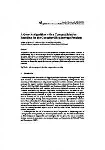
Programming, Branch and Bound and Dynamic Programming. Approximation optimisation algorithms are based upon constructive approaches (e.g. dispatching rules, etc.) and/or stochastic search techniques (e.g. Simulated Annealing, Taboo Search, Genetic Algorithm, Particle Swarm Optimization, Ant Colony Optimisation, Shuffled Frog Leaping and Artificial Immune Systems). Genetic Algorithms (GA) have several advantages. GA deal with a coding of the problem instead of decision variables (Syarif et al., 2002). They require limited domain knowledge (to represent the problem in terms of genes and chromosomes and also an objective function for evaluating the fitness of chromosomes) and use stochastic transition rules to guide the search (Goldberg, 1989). GA perform multiple directional search using a set of candidate solutions, whereas most conventional methods conduct single directional search (Gen and Cheng, 1997). There are many research articles related to GA and their applications in the fields of production and operations management. Aytug et al. (2003) reviewed more than 110 GA articles published between 1996~2002. They found that GA parameters and operators had mostly been selected in an ad hoc fashion, rather than using a systematic design of experiments approach. A survey conducted by Chaudhry and Luo (2005) stated that 67.98% of 178 GA related research articles had used GA to solve scheduling or facility layout problems. Much of the scheduling literature relates to classical job shop or flow shop problems and ignores assembly operations (Reeja and Rajendran, 2000). Multi-stage, multi-machine, multi-product scheduling (MMMS) is the allocation of resources over time to perform a collection of operations required by components, which are subsequently sub-assembled and assembled into products in accordance with the product structure. The number of levels of product structure indicates the number of stages of assembly precedence relationships. The leaf nodes within the product structure represent components. Since some components may require a number of operations to be performed on various machines, the sequence of operations for each component must consider the operation precedence constraint inherent its manufacturing process. Figure 1 shows an example of a typical product structure obtained from a collaborating company engaged in the capital goods industry. It can be seen that a final

Figure 1. A typical product structure from a collaborating company (Hicks and Pongcharoen, 2006).

206

Pupong Pongcharoen·Aphirak Khadwilard·Christian Hicks

product (P) required assemblies, subassemblies, parts and components (C), in each of which a sequence of operations (O) to be performed on multiple machines (M) is specified. In order to formulate the multi-stage, multimachine, multi-product scheduling (MMMS) model, the following notation is introduced for using in the model. Notation: i operation ith (i = 1, ⋯, O) j part or component jth (j = 1, ⋯, C) k final product kth (k = 1, ⋯, P) m machine mth (m = 1, ⋯, M) Rm ready time of machine mth (date) Ck completion time of product kth (date) Dk due date of product kth (date) Cjk completion time of component jth in product kth (date) Djk due date of component jth in product kth (date) Ek earliness duration of product kth (days) Ejk earliness duration of component jth in product kth (days) Tk tardiness duration of product kth (days) SUijkm setup time of operation ith for component jth in product kth on machine mth (minute) STijkm start time of operation ith for component jth in product kth on machine mth (minute) PTijkm processing time of operation ith for component jth in product kth on machine mth (minute) FTijkm finishing time of operation ith for component jth in product kth on machine mth (minute) TTijkm transfer time of operation ith for component jth in product kth on machine mth (minute) Xijkabcm 1 if operation ith for component jth in product kth precedes operation ath for component bth in product cth on machine mth; and 0 otherwise (minute) Pe earliness penalty (currency unit per day) Pt tardiness penalty (currency unit per day) S(x) set of child items of item x Sh working hour per shift (minutes per shift) The scheduling objective is based on the Just in Time philosophy that aims to minimise the combination of earliness penalties for components and final products and tardiness penalties of final products. The mathematical model for multi-stage multi-machine multi-product scheduling (MMMS) problem is as follows: Penalty cost C

=

P

∑∑ j =1 k =1

P

Pe( E jk ) +

∑

P

Pe( E k ) +

k =1

Subject to: STijkm ≥ Rm FTijkm = STijkm + SUijkm + PTijkm + TTijkm Cjk ≥ FTijkm Ejk = (Djk - Cjk)/Sh Ek = (Dk - Ck)/Sh

∑ Pt (T )

(1)

∀i, j, k, m ∀i, j, k, m ∀i, j, k, m ∀j, k ∀k

(2) (3) (4) (5) (6)

k

k =1

Tk = (Ck - Dk)/Sh ∀k STihkm - STijkm ≥ SUijkm + PTijkm + TTijkm ∀i, k, m, j∈ S(h) STgjkm - STijkm ≥ SUijkm + PTijkm + TTijkm ∀j, k, m, g = i + 1 ∀a, b, c, i, j, k, m Xijkabcm + Xabcijkm = 1 ∀a, b, c, i, j, k, m Xijkabcm ∈ {0, 1} Ejk, Ek, Tk ≥ 0 ∀j, k STijkm, Rm ≥ 0 ∀i, j, k, m FTijkm, STijkm, SUijkm, PTijkm, TTijkm ≥ 0 ∀i, j, k, m

(7) (8) (9) (10) (11) (12) (13) (14)

This mathematical model was derived to describe the MMMS problem considered in this research. The objective function (1) contains three parts: i) an earliness penalty for components; ii) an earliness penalty for final products; and iii) a tardiness penalty for final products. Constraint (2) ensures that the start time of all operations is not earlier than the time the machines are ready. Constraint (3) makes sure that the finishing time for each operation is determined by the start, setup, machining and transfer times. Constraint (4) ensures that the completion time for each component is not before the finishing time. The number of days earliness and tardiness for components and final products are defined by constraints (5), (6) and (7). Part precedence constraints relating to the product structure are defined by constraint (8). For example, if part j is child item of part h, then the start time of the parent part (STihkm) minus the start time of the child item (STijkm) should be greater or equal to the sum of setup, processing and transfer times for the child item. Constraint (9) makes sure that the operation precedence constraints within a component are satisfied. For example, if a successor operation (g) is performed after its predecessor operation (i) is finished, the start time of the successor operation (STgjkm) minus the start time of the predecessor operation (STijkm) should be greater or equal to the sum of setup, processing and transfer times of the predecessor operation. Constraint (10) ensures that only one operation can be performed on a machine using the decision variables defined by constraints in (11). Constraints (12)-(14) guarantee non-negative values for those defined variables. There is only limited research that relates to this multi -stage multi-machine multi-product scheduling (MMMS) problem. Pongcharoen et al. (2004) described a Genetic Algorithm tool that was developed for solving the MMMS problem and reported that the schedules obtained from GA outperformed the schedules obtained from a collaborating company. Pongcharoen et al. (2002) investigated the significance of the proposed repair process and found the best values for GA parameters using regression analysis. However, the computational experiments conducted in these papers ignored the genetic operations. The repair process used consisted of four steps: i) operation precedence adjustment; ii) part precedence adjustment; iii) timing assignment; and iv) deadlock adjustment. The part precedence adjustment was designed to satisfy product structure constraints i.e. an assembly requires all its subassemblies and components to be complete before it can


be produced. A deadlock situation may arise when there is a conflict between operation and part precedence constraints for different items that both require a common resource (Pongcharoen et al., 2002). Previous research relating to the multi-stage multimachine multi-product scheduling (MMMS) problem has not provided an exact mathematical formulation of the problem as outlined above. Chen and Ji (2007) applied a mixed integer programming method to solve a simple MMMS problem. Due to the limitation of their proposed method, the numerical experiments were based on a small-size problem that consisted of 2 final products with a requirement for 21 operations to manufacture 21 items (excluding final products). Some of the components were duplicated within the product structure. Each item only required one operation. Operation precedence constraints, setup and transfer times were ignored in their formulation.

207

coded into genes represented by alphanumeric strings. They had two parts: a part code (P) and an operation (O) number (see Figure 3). All the genes were randomly sequenced to generate a chromosome. This was repeated to generate a population of the specified size. It should be emphasized that the chromosome representation considered in this work was not separated into sub-chromosomes, which had been the approach adopted by previous research by the authors (Pongcharoen et al., 2002 and 2004). The undivided chromosome used was beneficial to the repair process that is described in the next sub-section.

3. GENETIC ALGORITHM FOR MMMS The Genetic Algorithm mechanism starts by encoding the problem to produce a list of genes. The genes are represented by either numeric (binary or real), or alphanumeric characters. Blazewicz et al. (1996b) suggested that the binary chromosome representation is often unsuitable for combinatorial optimization problems because it is very difficult to represent solutions. Therefore numeric or alphanumeric coding is often used. The next step is to randomly combine genes to produce a population of chromosomes, each of which represents a possible solution. Genetic operations (crossover and mutation) are next performed on chromosomes, which are randomly selected from the population as parents to produce offspring. A fitness function (objective function) is used to measure the chromosomes’ fitness value, from which the probability of their survival is determined. The most famous process is the ‘Roulette Wheel’ (Goldberg, 1989) which may also be used for chromosome selection. The GA process is repeated until a termination condition is satisfied. In this paper, the general Genetic Algorithm described by Goldberg (1989) was modified to include a new repair process for scheduling the manufacture of complex products in the multi-stage multi-machine environment. A schematic of the Genetic Algorithm based scheduling tool (GAST) is shown in Figure 2. It includes the following steps: i) chromosome presentation and initialisation; ii) a repair process; iii) fitness evaluation; iv) roulette wheel selection; v) a check of the termination conditions; and vi) genetic operations (crossover and mutation). The GAST program includes a graphic user interface and graphical outputs (e.g. Gantt charts). The program consists of nearly 10,000 lines of TCL programming language code (Ousterhout, 1994). 3.1 Chromosome Representation and Initialisation In this research the operations on each part were en-

Figure 2. Structure of the GA based Scheduling Tool (GAST).

Figure 3. Chromosome representation. 3.2 Repair Process The processes of chromosome initialisation and genetic operations within the evolution procedure within the GA may produce infeasible chromosomes (schedules) that represent impractical solutions that contravene constraints. There are three ways to deal with infeasible solutions: i) discard them; ii) apply a high penalty in the fitness function so that they are unlikely to survive; or iii) repair them (Blum and Roli, 2003). Discarding infeasible solutions or applying a high penalty is only an option when a large proportion of the population is feasible. Otherwise, the GA process could be terminated if all chromosomes in the population are infeasible. Several researchers have used a repair process for rectifying infeasible chromosomes in timetabling research (e.g. Caldeira and Agostinho, 1997; Colorni et al., 1998) and scheduling research (Pongcharoen et al., 2004). The re-

208


pair processes are problem specific due to differences between problem domains, chromosome representation, structures of the solution space and the nature of constraints. The undivided chromosome representation used in this work allowed a new compact repair process to be developed that has only two stages: i) part precedence adjustment; and ii) operation precedence adjustment. These processes are described in the following sub-sections. 3.2.1 Part Precedence Adjustment In previous research part precedence adjustment was based upon re-sequencing based upon the level of a part within the product structure. In this research part precedence adjustment was based upon the assembly lines defined in its product structure. For example, if there is a product structure (e.g. the product structure in Figure 3), part number 1, 2 and 3 require one operation whilst the remaining parts (part no. 4, 5, 6 and 7) require two operations. The process of checking and reordering parts was based on four assembly lines specified in the product structure. Figure 4 shows an example of checking and reordering parts in the first assembly line. The process began by selecting genes involved in the first assembly line for precedence checking regarding to the assembly line. If the selected genes had been in the wrong order (infeasible), then the selected genes are reordered based on its assembly requirement and finally replaced back to the positions they are selected but in a new feasible sequence. This process was repeated until all assembly lines in the product structure were considered.

For example, the product structure shown in Figure 3 has four parts (part no. 4, 5, 6 and 7) that required two operations for each part. Figure 5 shows an example of checking and reordering of the two operations required for part number 4. The genes corresponding to the operations on each part are identified and the order of operations is checked to ensure that is satisfies operation precedence constraints. If the selected genes are in the wrong order, then the selected genes are reordered in a new sequence. The process is repeated until the operation precedence constraints for all parts are satisfied.

Figure 5. Example of operation precedence adjustment. 3.3 Fitness Function The next stage was to measure the fitness of the chromosomes. The quality of schedules was evaluated by using the fitness (objective) function given in Equation (1), which aggregated the penalty cost arising from earliness and tardiness. 3.4 Roulette Wheel Selection This stage produced a new generation with the same population size as the initial population. The roulette wheel (Goldberg, 1989) approach was used for chromosome selection. It used a random number generator over the range 0-1 (Wichmann and Hill, 1982). The probability of survival and number of replicates of a chromosome in the next generation was determined by its fitness. The GA process was repeated until the termination criterion was satisfied.

Figure 4. Example of the new part precedence adjustment. The part precedence adjustment described allows the repair process to always avoid the deadlock situations that arose in previous research. This means that there was no conflict arising from operation and part precedence constraints. The deadlock adjustment was therefore excluded from the repair process proposed as it was unnecessary. The new repair process is therefore easier and requires fewer steps than those used in previous research. It is therefore more computationally efficient. 3.2.2 Operation Precedence Adjustment The process of operation precedence adjustment was applied to each part that required two or more operations.

3.5 Genetic Operations: Crossover and Mutation There are two types of genetic operator: crossover and mutation. A crossover operator generally combines the characteristics of two parents to produce an offspring, whilst mutation usually produces random change in one chromosome. Many crossover and mutation operators have been developed and reviewed in the literature (see for example Pongcharoen et al., 2001, which considered a comprehensive list). In this research, the nine crossover and nine mutation operators shown in Table 1 were considered. A Genetic Algorithm requires parameters and operators to be specified. There is no particular configuration that can guarantee to find the best solution for different problem sizes or domains. The configuration of GA struc-


ture should therefore be systematically investigated through using a design of experiments approach (Montgomery, 2001), which is described in the next section. Table 1. Crossover and mutation operators. Crossover operators (COP)

Mutation operators (MOP)

Enhanced edge recombination (EERX)

Enhanced 2-operation random swap (E2OR)

Order crossover (OX)

Inverse mutation (IM)

Partially mapped crossover (PMX)

Shift operation mutation (SOM)

Cycling crossover (CX)

Three operations adjacent swap (3OAS)

Position based crossover (PBX)

Three operations random swap (3ORS)

Maximal preservation crossover (MPX)

Two operations adjacent swap (2OAS)

One point crossover (1PX)

Two operations random swap (2ORS)

Two point centre crossover (2PCX)

Centre inverse mutation (CIM)

Mixed-crossover (MXOV)

Mixed-mutation (MMUT)

4. EXPERIMENTAL DESIGN AND ANALYSIS In this work, three sizes of industrial scheduling problem adopted from Pongcharoen et al. (2004) were considered (see Table 2). Data, including production schedules, product structure relationships, process plans and resource loading information were obtained from a

209

collaborating company that was in the make/engineer to order capital good industry. The first (small) problem, involved two different products (245 and 451), which had a combined requirement of twenty-five machining operations on eight resources with nine assembly operations. The second and third problems were termed medium and large, respectively. The large problem involved 118 machining and 17 assembly operations on 17 resources. There were interactions and contention for resources. The aim of the computational experiments was to investigate the performance of GA and to identify the best configuration of parameters and operators for the three problem sizes. The GA parameters and operators were considered as factors, each of which had three levels (see Table 3). The first factor was the combination of the population size and the number of generations (P*G), determined the total number of chromosomes (candidate solutions) created and therefore had a strong influence on the execution time. A large number of generations with a large population size increased the amount of search and increased the probability of finding an optimal solution. Due to the limitation of execution time and resources required for each computational run, the combination of P*G considered in this work was fixed at 2,500 chromosomes. The next two factors were the probabilities of crossover (%C) and mutation (%M). The range considered for these factors were adopted from previous research (Todd, 1997; Pongcharoen et al., 2002). Finally, nine crossover (COP) and nine mutation operations (MOP) shown in Table 1 were considered as last two factors. With these experimental factors and levels, a full factorial experimental design would require 2,187 (3x3x 3x9x9) computational runs for a single replication. In order to reduce this, a novel experimental design was

Table 2. Industrial scheduling problem. Problem number

Part number

1 2 3

245 and 451 229 and 451 4 and 228

Characteristics of scheduling problems Number of Products

Number of Components

Machining/Assembly Operation

Number of Resources

Levels of product structure

2 2 2

6 8 12

25/9 57/10 118/17

8 7 17

4 4 4

Table 3. Experimental factors and its levels. Factors

Levels

Propulation * Generation (P * G) Probability of Crossover (%C) Probability of Mutation (%M) Crossover operators (COP) Mutation operation (MOP)

3 3 3 9 9

Values Low (-1)

Medium (0)

High (+1)

25 * 100 0.1 0.05

50 * 50 0.5 0.1 See Table 1 See Table 1

100 * 25 0.9 0.15

210


adopted to reduce the number of runs required. The proposed design embedded a one-third (33-1) fractional factorial experimental design within the Latin Square experimental design. The factorial design (see Table 4) involved nine combination of treatments or settings denoted by the alphabet letters A, B, C, ⋯, I. Each combination was then embedded into the Latin Square design (see Table 5), which was based on the concept of a blocking experiment (Montgomery, 2001). It can be seen that each alphabet letter (treatment) was applied once and only once in each row (mutation) and column (crossover). Using the proposed experimental design, the total numbers of runs were reduced from 2,187 to 81 for each replication. This design dramatically reduced the computational effort by 96%. Experimental results were obtained from five replicates that used different random seed numbers. The results were then analysed using a general linear form of the analysis of variance and main effect plots were produced. Table 6 shows the F and p values for the main factors for each problem size. It can be seen that all the main factors were statistically significant with a 95% confidence interval as they had p values that were less than or equal to 0.05. However, P*G was statistically insignificant for medium problem. This means that the performance of GA

was dependent upon the configuration of the GA parameters and operators used. It should be noted that the average execution time were 20, 50 and 130 seconds for the small, medium and large problem, respectively (using a PC with AMD 1.3 GHz CPU with 128 MB RAM). Table 4. The one-third (33-1) fractional factorial design. Combine

P*G

%C

%M

U=0

A B C

25/100 25/100 50/50

0.1 0.5 0.1

0.05 0.15 0.1

000 012 101

D E F

100/25 25/100 50/50

0.1 0.9 0.5

0.15 0.1 0.05

202 021 110

G H

50/50 100/25

0.9 0.5

0.15 0.1

122 211

I

100/25

0.9

0.05

220

In order to identify the appropriate settings of the significant parameters, main effect plots for the statistically significant parameters are presented in Figure 6. It can be seen that, for the small problem, the best results

Table 5. The Latin Square design. Design

CX

EERX

MPX

IPX

OX

PBX

PMX

2PCX

MOXV

2OAS 3OAS 2ORS 3ORS IM SOM CIM

A B C D E F G

I A B C D E F

H I A B C D E

G H I A B C D

F G H I A B C

E F G H I A B

D E F G H I S

C D E F G H I

B C D E F G H

E2ORS MMUT

H I

G H

F G

E F

D E

C D

B C

A B

I A

Table 6. The analysis of variance on three problem sizes. Problem sizes Medium

Small

Large

Source

DF

F

P

F

P

F

P

P*G %C %M COP MOP Seed Error Total

2 2 2 8 8 4 378 404

36.46 4.46 3.09 8.17 4.71 4.82

0.000 0.012 0.047 0.000 0.000 0.001

1.99 22.31 2.87 35.21 2.67 16.8

0.138 0.000 0.058 0.000 0.007 0.000

13.29 21.56 7.64 40.14 2.81 19.27

0.000 0.000 0.001 0.000 I0.005 0.000


were obtained from the setting of P*G at 100*25 with the probabilities of crossover and mutation set at 0.5 and 0.15 respectively. For the medium problem, the best configuration was 50*50, 0.9 and 0.1, respectively. Whilst the best setting for the large problem was found to be at 50*50, 0.9 and 0.1, respectively. These results indicated that the best GA configurations are problem specific and are influenced by the structure of the problem domain, the size of the solution space and the nature of the constraints.

211

mutation, the appropriate operators were 3ORS, CIM and MMUT. It can be concluded that the efficiency of GA operators were differentiated according to the size of the scheduling problem.

(a) Small problem

(a) Small problem

(b) Medium problem

(b) Medium problem

(c) Large problem

Figure 7. Main Effect Plot of the GA operators.

(c) Large problem

Figure 6. Main Effect Plot of the GA parameters. Main effect plots for both statistically significant operators are presented in Figure 7. This suggested that the best crossover operators for small, medium and large size problems were MPX, MPX and OX respectively. For

Even though the efficiency of the GA operators was different for the various problem sizes considered, it was worth investigating which operator generally performed best. Table 7 shows the mean and standard deviation of the penalty costs associated with the schedules obtained for the different problems. When considering the best and the second best performance of both crossover and mutation operators for each problem sizes, the maximal preservation crossover (MPX) and the mixed mutation (MMUT) operators were found to help the GA process to achieve the lowest mean penalty costs.

212


Table 7. The mean and standard deviation of COP and MOP. Small Mean

SD

Medium Mean

Large SD

Mean

SD

Crossover 1PX

15411(6)

937

57000(6)

2284

199811(5)

4571

2PCX CX EERX

15500(7) 15589(8) 15067(2)

1034 1083 252

57100(7) 57400(8) 52933(2)

1718 1938 3715

200122(7) 201956(8) 194744(3)

4111 3834 4279

MPX

229

193922(2)

6449

294 360 1283

51511(1) 55622(4) 54656(3) 57667(9)

5230

MXOV OX PBX

15067(1) 15100(3) 15133(4) 15956(9)

1995 2840 1822

196789(4) 193167(1) 202356(9)

3677 4430 3837

PMX

15356(5)

889

56911(5)

1923

200000(6)

3999

15678(9) 15356(6) 15511(7)

1262 816 1084 126 529 1207 229 420 886

55689(5) 55978(7) 56667(9) 55633(4)

2859 2650 2527 2647 5075 4068 2130 3841 4243

198944(8) 199244(9) 198433(6) 197533(3) 197189(2) 198878(7) 198133(4)

5055 4615 5735 5338 6876 5651 4215 6202 5112

Mutation 2OAS 2ORS 3OAS 3ORS CIM E2ORS IM MMUT SOM

15033(1) 15244(4) 15678(8) 15144(2) 15211(3) 15322(5)

5. CONCLUSIONS This paper described the Genetic Algorithm based Scheduling Tool (GAST) for solving the multi-stage multi-machine multi-product scheduling (MMMS) problem. A mathematical model of MMMS problem was proposed. The model considered setup and transfer times and the operation precedence constraints within each component, which had been ignored by previous research. The proposed algorithm included a new repair process that was embedded within the proposed GA for rectifying infeasible schedules that were generated in the evolution process. A new repair process was used that always avoided deadlock, which was a problem in previous research. The algorithm minimises the combination of earliness and tardiness penalties with finite resource capacity. The GAST was applied to solve three representative problems obtained from a collaborating capital goods company. The computational experiments were aimed to investigate the appropriate settings of Genetic Algorithm parameters and mechanisms for various problem sizes using an advanced experimental design. The proposed design dramatically decreased the computational time and computing resource required. The analysis of experimental results obtained from the GAST indicated that all the Ge-

54900(1) 55756(6) 56200(8) 54944(2) 55033(3)

196367(1) 198144(5)

netic Algorithm parameters and mechanisms influenced the results obtained for all three problem sizes. However, the efficiency of crossover and mutation operators varied depending on the problem size. It suggested that the appropriate setting of GA parameters and mechanisms were dependent on the size and the structure of the solution space, which was directly related to the problem size.

REFERENCES Aytug, H., Khouja, M., and Vergara, F. E. (2003), Use of genetic algorithm to solve production and operation management problems: a review, International Journal of Production Research, 41, 3955-4009. Baker, K. R. (1974), Introduction to Sequencing and Scheduling, Wiley and Sons, New York. Blazewicz, J., Domschke, W., and Pesch, E. (1996a), The job shop scheduling problem: Conventional and new solution techniques, European Journal of Operational Research, 93, 1-33. Blazewicz, J., Ecker, K. H., Pesch, E., Schmidt, G., and Weglarz, J. (1996b), Scheduling Computer and Manufacturing Processes, Springer, Berlin. Blum, C. and Roli, A. (2003), Metaheuristics in combina-


torial optimisation: overview and conceptual comparison, ACM Computing Surveys, 35(3), 268-308. Caldeira, J. P. and Agostinho, C. R. (1997), School timetabling using genetic search, Proceedings of the Practice and Theory of Automated Timetabling, University of Toranto, Toronto, 115-122. Chen, K. and Ji, P. (2007), A mixed integer programming model for advanced planning and scheduling (APS), European Journal of Operational Research, 181(1), 515-522. Chaudhry, S. S. and Luo, W. (2005), Application of genetic algorithms in production and operation management: a review, International Journal of Production Research, 43, 4083-4101. Colorni, A., Dorigo, M., and Maniezzo, V. (1998), Metaheuristics for high school timetabling, Computational Optimisation and Application Journal, 9, 277298. Fry, T. D., Oliff, M. D., Minor, E. D., and Leong, G. K. (1989), The effects of product structure and sequencing rule on assembly shop performance, International Journal of Production Research, 27, 671-686. Gen, M. and Cheng, R. (1997), Genetic Algorithms and Engineering Design, John Wiley and Sons, New York. Goldberg, D. E. (1989), Genetic Algorithms in Search, Optimisation and Machine Learning, AddisonWesley, Reading, MA. Garey, M., Johnson, D., and Sethi, R. (1976), The complexity of flow shop and job shop scheduling, Mathematics of Operations Research, 1(2), 117-129. Graham, R., Lawler, E., Lenstra, J., and Rinnooy K. A. (1979), Optimisation and approximation in deterministic sequencing and scheduling: a survey. Annals of Discrete Mathematics, 5, 287-326. He, Y. and Hui, C. W. (2007), Genetic algorithm based on heuristic rules for high-constrained large-size single stage multi-product scheduling with parallel units, Chemical Engineering and Processing, 46(11), 1175 -1191. Hicks, C. and Pongcharoen, P. (2006), Dispatching rules for production scheduling in the capital goods industry, International Journal of Production Economics, 104(1), 154-163. King, J. R. and Spackis, A. S. (1980), Scheduling: bibliography and review, International Journal of Physical Distribution and Materials Management, 10,

213

105-132. Montgomery, D. C. (2001), Design and Analysis of Experiments, Fifth edition, John Wiley and Sons, NY. Nagar, A., Haddock, J., and Heragu, S. (1995), Multiple and bicriteria scheduling: a literature survey, European Journal of Operational Research, 81, 88-104. Ousterhout, J. K. (1994), Tcl and the Tk Toolkit, Addison Wesley, Massachusetts. Pongcharoen, P., Stewardson, D. J., Hicks, C., and Braiden, P. M. (2001), Applying designed experiments to optimise the performance of genetic algorithms used for scheduling complex products in the capital goods industry, Journal of Applied Statistics, 28(3-4), 441455. Pongcharoen, P., Hicks, C., Braiden, P. M., and Stewardson, D. J. (2002), Determining optimum genetic algorithm parameters for scheduling the manufacturing and assembly of complex products, International Journal of Production Economics, 78(3), 311-322. Pongcharoen, P., Hicks, C., and Braiden, P. M. (2004), The development of genetic algorithms for the finite capacity scheduling of complex products, with multiple levels of products structure, European Journal of Operational Research, 152(1), 215-225. Reeja, M. K. and Rajendran, C. (2000), Dispatching rules for scheduling in assembly job shops-Part I, International Journal of Production Research, 38(9), 2051 2066. Reisman, A., Kumar, A., and Motwani, J. (1994), Flowshop scheduling/sequencing research: a statistical review of the literature, 1952~1994, IEEE Transactions on Engineering Management, 44(3), 316-329. Ruiz, R. and Maroto, C. (2005), A comprehensive review and evaluation of permutation flow shop heuristics, European Journal of Operational Research, 165, 479 -494. Syarif, A., Yun, Y., and Gen, M. (2002), Study on multistage logistic chain network: a spanning tree-based genetic algorithm approach, Computers and Industrial Engineering, 43(1-2), 299-314. Todd, D. (1997), Multiple Criteria Genetic Algorithms in Engineering Design and Operation, Ph.D. thesis, Faculty of Engineering, University of Newcastle upon Tyne, UK. Wichmann, B. A. and Hill, I. D. (1982), Algorithm AS 183 an efficient and portable pseudo-random number generator, Applied Statistics, 31, 188-190.