a glimpse into poisson regression model and its ...

Int. J. Agricult. Stat. Sci., Vol. 10, No. 1, pp. 83-91, 2014

ISSN : 0973-1903

ORIGINAL ARTICLE

A GLIMPSE INTO POISSON REGRESSION MODEL AND ITS FURTHER DEVELOPMENTS Jiten Hazarika* and Irani Saikia Department of Statistics, Dibrugarh University, Assam, India. E-mail : [email protected] Abstract : The Poisson regression model, a member of the family of Generalized Regression models, provides a standard framework for the analysis of count data, which are common in applied research. Given the widespread use of regression model for count data, the purpose of this paper is to give a critical review on research works for Poisson regression model as the bench mark model in the analysis of count data, its further developments and on its competitors like negative binomial regression model and Cox regression model. An application to infant mortality data illustrates superiority of Poisson regression model over the logit regression model. Key words : Generalized Poisson regression, Zero inflated Poisson regression, Bi-Variate Poisson regression

1. Introduction Poisson regression model, a standard model for analysis of count data, is a member of the generalized linear models- a class of models, which encompasses both normal linear regression models and also the nonlinear counterpart. The generalized linear models, which represent a family of statistical techniques that can be used to analyze a wide variety of research problem was proposed by Nelder and Wedderburn (1972). Each member of this class is a univariate model as it predicts or model the behavior of one particular variable (response variable, explained variable) and the key assumption is that the response variable distribution is a member of the exponential family of distributions. Thus, this family of models is characterized by (i) A dependent variable z whose distribution with parameter .... is one of the class in (z;,)=exp[() {z–g() + h(z)} + (, z)], where, () > 0, so that for fixed , we have an exponential family. The parameter  could stand for a certain type of nuisance parameter such as the variance 2 of a normal distribution. (ii) A set of independent variables x1, x2, ..., xm and predicted yi = i xi , where i ’s are parameters, whose values may be fixed (known) or unknown and require estimation. (iii) A linking function  = f (y) connecting the parameter  of the distribution of z with the y's of the linear model. *Author for correspondence.

Received October 11, 2013

When z is normally distributed with mean  and variance 2 and when  = y, it represents ordinary linear models with normal errors. The generalized linear models include exponential, logistic and Poisson regression models as well as many other models, such as, log-linear model for categorical data. Any regression model that belongs to the family of generalized regression models can be analyzed in a unified fashion. The maximum likelihood estimates of the regression parameters can be obtained by iteratively reweighted least squares. The benefit of use of this class of models is that here, fulfilment of the assumption of normality and constant variance is not mandatory. However, a general linear model is a special case of generalized linear regression. In this paper, emphasis is given on Poisson regression model with a real life application and its further extensions.

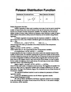
2. Poisson Regression Model & its Application Poisson or count data model focuses on the number of occurrences of an event. Here, the outcome variable is y = 0, 1, 2, … and the probability distribution used is Poisson. i.e.  yi ~ p(µi ), yi = 0, 1, 2, ... with E{yi } = µi  The mean response is a function of the linear predictor variables Xi1, ..., Xip–1 and is denoted by X i'    0  1 X i1  ... p 1 X ip 1  µ(Xi , ) is the function that relates the mean response µi to Xi (values of the predictor variables Revised March 21, 2014

Accepted April 15, 2014

84

Jiten Hazarika and Irani Saikia

for case i) and (values of the regression coefficient).

c

h

Poisson regression function µi = µ(Xi , ) = log X i' , is

c h

In the multiple logistic regression model,

 *  log X i' ,b .

c h , where y is independent E ly q    1  expc X  h

After parameter estimation, the basic idea of the members of the GLM is to develop a linear model for an appropriate function of the expected values of the response variable and to draw inferences. The inferences in Poisson regression models are drawn as in case of logistic regression.

exp X i' 

i

i

i

' i

Bernoulli random variables. Then the logistic transformation = log

FG  IJ , here H1   K i

i

FG  IJ is odds and the link function H1   K F  IJ  X  gb g  logG H1   K i

i

' i

i

i

i

So, if y i ~ p(µ i ), then, the response function

c h

 i  exp X i'  . Thus, g(µi ) = loge(µi ) = X i' , which is the link function for Poisson regression. Thus, the Poisson regression model under the log link function is Loge(µi ) = 0 + 1Xi1+...+p–1Xip–1   i  e

 0   j X ij

, i = 1, 2, … n and j = 1, 2, …, p-1

The likelihood function is

bg

b

 Xi ,

n

L  

g

yi

b

exp   X i , 

g

Yi !

i=1

RS b X ,g UV expLM  X , OP W N Q T n

n

yi

i

i

i=1

i=1

n

 Yi ! i=1

bg

n

b g

n

b g

n

b g

Log L    Yi log  X i ,     X i ,    log e Yi ! i=1

i=1

i=1

To find the maximum likelihood estimates of the parameters  0 ,  1 , …,  p-1 , numerical maximization procedures can be utilized. These estimates can be obtained through reweighted least squares. Now-a-days various statistical software packages like R, S-plus, SPSS are also available to obtain the maximum-likelihood estimates. From these estimates, the fitted response function and fitted values can be obtained and thus the fitted response function and the fitted values for the

The Poisson regression model is often applied to study the occurrence of small numbers of counts or events as a function of a set of predictor variables, in experimental and observational studies and also in many disciplines including economy, demography, psychology, medicine and also in insurance sector. In epidemiology, these models are used to investigate the occurrence of selected diseases in exposed and unexposed subjects in observational prospective studies. After the developments of GLM in 1972, these were extensively developed by Mc. Cullagh and Nelder (1989). However, in the meantime, Coale and Trussel (1974) developed a fertility model known as Poisson regression model for Coale-Trussel parameter. Poisson regression can also be applied to panel data as suggested by Hausman et al. (1984). Cameron et al. (1986) applied this model in health demand studies. The Poisson regression model and some other models of the family of GLMs like the negative binomial regression have become indispensable tool in applied research for count data. These standard techniques are used in various studies like, discovery of new drugs [Jensen (1987)], studies on trip frequencies suggested by Rickard (1988) and Barmby and Doornik (1989), violations of safety regulations [Feinstein (1989)] and escape clause petitions by Coughlin et al. (1989) etc. Even the annual number of bank failures over some period may be analyzed by using Poisson regression by taking explanatory variables such as bank profitability, corporate profitability and bank borrowings from the Federal Reserve Bank as suggested by Davutyan (1989). Various rates like, recruitment rates [Kostiuk and Follmann (1989)], offer arrival rates [Ember (1990)], market entry [Chappell et al. (1990)] etc. that apply count data were also done by using Poisson regression model. Again, accident analysis studies model airline safety for example, the number of accidents experienced by an airline over some period and interested to find out its relationship to airline profitability and other measures of financial health of the airline [Rose (1990)] was also done using Poisson regression model. The examples of the application of this standard model are available from micro

A Glimpse into Poisson Regression Model and its Further Developments

econometrics also like, fertility studies often model the number of live births over a specified age interval of mother, with interest in analyzing its variation in terms of say, mother ’s schooling, age, household income etc [Winkelmann (1995)]. Gurmu and Trivedi (1996) suggested the use of Poisson regression model in modeling the number of trips to a recreational site to place a value on natural resources such as national forests etc. Cameron and Trivedi (1998) covered basics to application of count data regression model in analyzing event data. Nicola et al. (2000) published a paper on spatial Poisson regression for health and exposure data. Wiper et al. (2001) developed reliability modeling using metric information for software in Bayesian inference. There, they were concerned with predicting the number of faults N and time to next failure of a piece of software. Information in the form of software matrices data is used to estimate the prior distribution of N through a Poisson regression model. The specific merits of the Poisson regression model are: it captures the discrete and non-negative data and allows drawing inferences on the probability of event occurrence. The model may also be used as an alternative to Cox model for survival analysis, when hazard rates are approximately constant during the observation period and the risk of the event under study is small (e.g. incidence of rare diseases) [Breslow and Day (1987)]. Again in ecological investigations, where the aggregated form of data is available like the count, the Cox model can be replaced by Poisson regression. Ma et al. (2003) introduced a Poisson regression modeling approach to random effects Cox models.

3. An Application This application attempts to model relationship between infant mortality in Assam and its probable predictors using Poisson and Logistic regression model. In such type of studies, the widely used model is the Logit regression model. But, now-a-days general decline trend in the infant mortality has created renewed interest in the factors behind and causes of infant mortality using Poisson regression model. Keeping this point in view, an empirical investigation has been carried out to compare efficiency of Logit and Poisson regression models in predicting impact of some socio-economic and demographic factors on infant mortality among the women in Assam. The variables used in this modeling have been explained in Table 1. Table 2 depicts results obtained by fitting Poisson regression model whereas the results of the estimated logistic regression model are presented in Table 3.

85

Comparing AIC and BIC of both the models, it is observed that the Poisson regression model is better than the logit model. In case of Poisson regression, the value of model deviance and Pearson Chi-square are 0.750 and 1.406, respectively. As these values are not so far distance from 1 the fitting of Poisson regression model is quite satisfactory. This study establishes superiority of Poisson regression model over the logit model. This illustration as well as the literatures cited above necessitates the use of the Poisson regression model while dealing with count data. But this model is not suitable while dealing with data having overdispersion and underdispersion. Under these situations, the Generalized Poisson (GP) regression model and the Negative Binomial (NB) models can be the alternatives.

4. Generalized Poisson Regression Model The specific assumptions of Poisson regression model are: the intensity of Poisson process is a deterministic function of the covariates and the events occur randomly over time. But in most of the economic phenomena, such assumptions are suspicious and in applications it is not always possible to realize the equality [Frome et al. (1973), Agresti (1997), Bohning et al. (1998), Cameron and Trivedi (1998), Stokes et al. (2000), Banik and Kibria (2008)] and lead to the violation of Poisson variance assumption. Thus, while dealing with situations like overdispersion or underdispersion, i.e. when the sample variance is larger (or smaller) than the sample mean, the Poisson regression model causes biased parameter estimation [Cox (1983)]. When there is overdispersion in the data set, it is better to use GP regression models [Lawles (1987), Ridout et al. (2001), Jansakul (2005), Kibria (2006), Long and Freese (2006)]. In order to overcome the problem of overdispersion, researchers like Famoye (1983), Lawless (1987) employed the NB and GP regression models instead of Poisson regression. Cameron and Trivedi (1998) and Winkelmann (2003) did excellent survey on overdispersion and its treatment. According to Famoye et al. [2004], if the data type is known i.e., if the data is overdispersed, then either the NB regression model or the GP regression model can be used, but, if the type of the dispersion is unknown, then the choice should be GP regression model as it is more flexible. The probability function of GP regression model is:

F  IJ FG 1+  IJ f (y ;µ ,x)= G H 1+  K H y ! K yi

i

i

i

i

i

i

i

yi  

exp

LM  b1+ y g OP N 1+  Q i

Here, yi = 0, 1, 2, …; µi = µi (xi ) = exp(xi , )

i

i

86

Jiten Hazarika and Irani Saikia

Where, xi is a (k-1) dimensional vector of covariates and  is a k dimensional vector of regression parameter. The mean and variance of y are

b

E yi xi   i and V yi xi   i 1   i

g

2

When the parameter  = 0, then GP regression reduces to Poisson regression model. Thus, the GP regression model is a generalization of the standard Poisson regression model. Famoye et al. (2004) applied both Poisson regression model and GP regression model to the accident data. But, the paper resulted that modeling overdispersed data using GP regression model is more appropriate than Poisson regression model. They came into this decision after observing the log-likelihood values for both the models. There may be many situations, where the data generating process results into too many zeros. Count data with too many zeros are very common in a number of applications. In such situations, the Zero-Inflated Poisson (ZIP) regression models are used instead of Poisson regression and GP regression.

5. Zero Inflated Poisson Regression Model & its Extensions The ZIP regression models were originated in the econometrics literature [Mullahy (1986)], but it has become more widespread since the publication of Lambert (1992). Lambert described the ZIP regression models with an application to defects in manufacturing. In that work, he explained that these models are not only easy to interpret but they can also lead to more refined data analyses. In the experiment concerning soldering defects on printed wiring boards that not only gives the mean number of defects but also why the means are lower. In order to explain the extra zeros in the variable, the ZIP regression is

b

g

b

g b g = b1   g expb   g  y !, y  0

p yi xi   i  1   i exp   i , yi  0 i

i

yi i

i

i

Here, i represents the probability of the existence of extra zeros. Bohare and Krieg (1996) used a ZIP regression model to handle the mover-stayer problem in demography. In a study made by Greene (1997) found that, the ZIP models are relatively common among econometrician in insurance industry. Besides this Ridout et al. (1998) cited examples of data with too many zeros from various disciplines including agriculture, econometrics, patent applications, species abundance, medicine and use of recreational

facilities. The ZIP regression model assumes that the population consists of two different types of observations. The first is based on zero counts while the second has a Poisson distribution [Bohning (1999)]. He found that the regression models are useful in the study of the number of decayed, missing or filled teeth. The ZIP regression model has been applied in various disciplines including horticulture [Hall (2000)], health operations [Wang and Famoye (1997)] and thus it experienced a wide-spread popularity. Cheung (2002) used a ZIP regression analysis to study the growth & development. Wikle and Anderson (2003) used this model to model the count observations of meteorology. Famoye and Ilknur (2007), Minami et al. (2007) developed count regression model with applications to Zoological data containing structural zeros. Prior to this, Yau and Lee (2001), Ridout et al. (2001), Lee et al. (2001), Martin et al. (2005) also used ZIP regression model to model data having too many zeros. The Zero-Inflated Binomial (ZIB) and Zero-Inflated Negative Binomial (ZINB) regression models are strong competitors of ZIP regression model. The ZIP regression model is especially useful in analyzing count data with large number of zero observation, however, in practice the ZIB model is sometimes used for cases in which the upper bound for the response exists. The ZINB model is used for overdispersed data. In the study made by Karazsia and Dulmen (2008) on childhood injury, they compared Poisson regression, Negative Binomial, ZIP, ZINB, on that data, found that ZIP best suit the observational data. Abdullah et al. (2010) used the ZIP models in order to model insect-egg data with excess zeros. Recently, Wildhaber et al. (2011) used ZIP regression model in fisheries biology. In the year 1969, Johnson and Kotz developed a model and Mullahy (1986) first used a model in econometrics by allowing for regression effects. This model is known as hurdle model. The basic idea for a hurdle model was developed by Cragg and Uhler (1970) as a modification of Tobit model. Cragg's specification of this modified Tobit model was employed as a basis of test of the Tobit specification by Lin and Schmidt (1984). These models are useful for count data of “too many” or “too few” zeros compared to the Poisson model. The hurdle Poisson model allows for a systematic difference in statistical process governing observations with zero counts and observations with one or more counts. It is a compound Poisson model as it is the combination of dichotomous model governing binary outcome of the count being zero or positive and truncated (situations, where data are observed only over part of the range of the response variable) at zero-Poisson model for strictly positive outcomes. The hurdle at zero model

A Glimpse into Poisson Regression Model and its Further Developments

addresses any situation, in which, there are more (overdispersed) or less (underdispersed) zeros in the data than predicted by Poisson model. The hurdle model [Winkelmann and Zinmermann (1991)] is P(Y = 0) = f1(0)

b

g b g 11  ff bb00gg

P Y  y  f2 y

1

2

the method of maximum likelihood. In ZIGP distribution, the zeros are assumed to occur in two distinct states. In the first state, the zeros occur with probability pi called “structural zeros” and in the second state with probability (1–pi) and leads to Generalized Poisson distribution with dispersion parameter  and µi. These zeros are called “sampling zeros”. The general form of ZIGP regression model is

b

bg

Gupta et al. (1996) proposed the use of the Zeroadjusted Generalized Poisson model to analyze overdispersed fetal movement data and death notice of data of London Times. Count data often exhibit overdispersion and/ or require an adjustment for zero outcomes with respect to Poisson model. Dietz and Bohning (2000) first introduced the zero modified Poison regression (ZMP) models. In order to test the misspecification in count regression models, score tests score widely used as they require null-hypothesis to fit the model. In the score test for ZI, there is confusion with regard to the limiting distribution of score test statistics or the interpretation of rejecting the null-hypothesis. The ZI parameter  is interpreted as the probability of getting a zero-outcome. But ZI distributions are characterized by small negative values of the parameter . Thus, these negative values correspond to zero deflation. Thus, the score test now has two sided alternative hypotheses,  0 :   0 against  1 :   0. Thus, the null- hypothesis is to be rejected based on both ZI and zero deflated not only on ZI, i.e. in favour of zero modification. Min and Czado (2003) introduced the Zero Modified Generalized Poisson (ZMGP) as an extension over ZMP regression models. Famoye and Singh (2006) extended the work of Gupta et al. (1996) to a more general situation, where the count dependent variable is affected by some co-variate. They noted cases, where the ZIP models were inadequate and ZINB regression model could not be fitted to an observed data set. This realization motivated them to develop a Zero-Inflated Generalized Poisson (ZIGP) regression model for modeling overdispersed count data with too many zeros. They applied this model first to domestic violence data. They estimated the proposed model using

gb

g

P Y  yi xi , Zi  Pi  1  Pi  , ,0 , yi = 0

= (1 – Pi ) f(µ1, ; 0)

 f 2 y , y = 1, 2, ....

Where, f1 and f2 are any probability distribution function for positive integers. The numerator of  gives the probability of crossing the hurdle and denominator of is normalization for f2.

87

Where, f (µi , ; yi), yi = 0, 1, 2, … is the GP regression model. The mean and variance of ZIGP regression models are

b g b g b g V bY X g  b1  P g    b1   g  b1  P g  = E Y X b1   g  P  E Yi X i  1  Pi  i X i and i

i

2 i

i

2

i

2

i

i

2 i

2

i

i

i

i

i

When Pi = 0, this ZIGP regression model reduces to GP regression model and when  = 0, it reduces to ZIP regression model. Moreover, if Pi is positive, it represents ZIGP regression model and if Pi is negative, it represents Zero deflated generalized Poisson regression model. The ZIGP regression is a large class of regression models, which contains ZIP, GP and Poisson regression [Mullahy (1986), Lambert (1992), Consul and Famoye (1992), Famoye (1993)]. The ZIGP regression have found useful for analysis of count data with a large amount of zerocount [Famoye and Singh (2003), Gupta et al. (2004), Joe and Zhu (2005), Bae et al. (2005)]. In their work, Famoye and Singh (2006) compared ZIGP, with ZIP and GP regression in domestic violence data and found that ZIGP regression model are more appropriate for this. Czado et al. (2007) introduced flexible ZIGP regression models and applied to patent outsourcing rates. They found that flexible ZIGP is more superior than GP, ZIP and even to ZIGP regression. In all these above cases, the count data regression models focus on univariate cases, where the single dependent variable takes the non-negative integer. However, situation may demand to jointly estimate two count independent variables, which are correlated. This situation can be handled by bivariate count models. These models analyses correlated events like: the number of doctor visit and non-doctor professional visit; the number of visits to the general practitioners and visits to

88

Jiten Hazarika and Irani Saikia Table 1 : Description of Explanatory Variables. No.

Variable

Type

Socio economic variables 1.

Educational status

Categorical with nominal scale (Literate (0), Illiterate (1))

2.

Residential status

Categorical with nominal scale (Urban (0),Rural (1))

3.

Socio economic status

Categorical with ordinal scale (Higher (0), Middle (1), Lower (2))

Demographic variables 4.

Age of mother at her 1st birth

Categorical with nominal scale (19-35(0),35(1))

5.

Caste

Categorical with nominal scale (Others (0), ST (1), SC (2))

Table 2 : Results of Multiple Poisson Regression Model. Characteristics



S.E.

Wald Chi square

d.f

P- value

Rate Ratio exp ()

Intercept

-2.637

.1855

201.995

1

.000

.071

Lower .049

Upper .103

1

.000

1.693

1..282

2..236

Educational Status Illiterate

95.0% C.I. for rate ratio

Literate(r) .527

.1417

Caste

13.812 Others(r)

SC

-.375

.2177

2.974

1

.085

.687

.448

1.052

ST

-.062

.1639

.144

1

.704

.939

.681

1.295

Socio Economic Status

Higher(r)

Lower

.683

.2079

10.787

1

.001

1.979

1.316

2.974

Middle

.674

.1929

12.194

1

.000

1.962

1.344

2.863

1

.109

1.303

.942

1.800

1

.008

1.410

1.094

1.820

Rate Ratio exp ()

95.0% C.I. for rate ratio

Residential Status Rural

Urban(r) .265

.1651

Age of Mother at Her First Birth < 19 and >35

.344

2.575 19-35(r)

.1298

7.029

AIC = 684.76

BIC = 694.97

Table 3 : Results of Multiple Logistic Regression Model. Characteristics Intercept



S.E. -2.763

.177

Educational Status Illiterate

Wald Chi square

d.f

P- value

242.484

1

.000

.063

1

.000

.009

1

2.831

Lower

Upper

1.697

1.270

2.268

.923

.984

.706

1.372

1

.092

.690

.448

1.063

Literate(r) .529

.148

Caste

12.787 Others(r)

SC

-.016

.170

ST

-.371

.220

Socio Economic Status

Higher(r)

Lower

.737

.204

13.056

1

.000

2.090

1.343

3.118

Middle

.662

.187

12.476

1

.000

1.938

1.401

2.798

.284

.166

1

.087

1.328

.960

1.838

1

.006

1.445

1.111

1.881

Residential Status Rural

Urban(r)

Age of Mother at Her First Birth < 19 and >35

.368

2.938 19-35(r)

.134

AIC = 1528.32 Note: 'r' represents reference category.

7.521

BIC = 1538.52

A Glimpse into Poisson Regression Model and its Further Developments

specialists; the number of insurance claims with and without bodily injuries.

6. Bivariate Poisson Regression As mentioned above if (y1, y2) is paired data, the Bivariate Poisson Regression for (y1, y2) [Holgate (1964), Paul and Ho (1989), Kocherlakota and Kocherlakota (1992)] is

In real life, there are many situations where the conventional Poisson regression model may not be satisfactory (appropriate) to use. Under this situation, the following are the alternatives originated from benchmark model for count data, viz. Poisson regression model. ●

f(y1, y2 / 0, 1, 2) = exp(–1 –2 –0)

l

min y1 , y 2

×

 i 0

q

 1y i  2y i  i0 y1  i ! y2  i !i! 1

b

2

gb

g

●

Where, E(Y1) = 1 + 0 and E(Y2) = 2 + 0 and cov(Y1 + Y2) = 0. Li et al. (1999) focus on the bivariate case, by deriving a Bivariate ZIP (BivZIP) distribution as mixture of two univariate Poisson distributions. In order to estimate these models, they used maximum likelihood. Wang et al. (2003) used a bivariate ZIP regression model to analyze two types of occupational injuries. Lee et al. (2005) further developed a bivariate ZIP regression model to analyze same occupational injuries data. Jiang and Paul (2009) proposed a Zero-Inflated Bivariate Poisson (ZIBP) regression model in order to analyze the data that are in the form of paired counts. In that paper the researchers used the ZIBP regression model to paired (pre-treatment and post-treatment) dental epidemiological counts. Mazumder et al. (2010) extended the work of Li et al. (1999) and proposed a Bayesian BivZIP regression model with estimation based on data argumentations. Arab et al. (2011) proposed a semiparametric ZIP modeling approach for bivariate count process, which extends the existing Bivariate Zero-Inflated modeling approaches to utilization of non-linear covariates in the model as well as modeling Zero-inflation probabilities through a multinomial logit regression. Likewise, various developments are made and still it is going on.

7. Concluding Remarks While dealing with count data the Poisson regression model is one of the foremost candidates among the family of GLM. The Poisson regression model may be used as an alternative to Cox model for survival analysis, when hazard rates are approximately constant during the observation period and the risk of the event under study is small. Again in ecological investigations, where the aggregated form of data is available like the count, the Cox model can be replaced by Poisson regression. In our work, an empirical investigation has also been carried out using Poisson as well as logit regression models which, establishes superiority of the former compared to the latter.

89

●

●

If the variance of the data exceeds (less than) the mean, which is referred to as extra-Poisson variation or overdispersion (underdispersion) relative to Poisson model, then the situation calls for a more general model, i.e. Generalized Poisson regression model. If the data type is known i.e. if the data is overdispersed, then either the NB regression model or the GP regression model can be used, but, if the type of the dispersion is unknown, then the choice should be GP regression model as it is more flexible. If the observed data show a higher relative frequency of zeros, or some other integer, than is consistent with the Poisson model then, this problem can be handled by the Zero-inflated Poisson regression model. If the observed data show both overdispersion as well as excess zero problem, then the Zeroinflated Generalized Poisson regression is applicable to such count data.

If the two count independent variables are correlated, then to jointly estimate them, the Bivariate count (bivariate Poisson) models are applicable. Further depending upon situations, BivZIP can be utilized. Inspite of these, the Poisson regression model and its other developments remain partly poor known, especially if compared to other regression techniques like linear, logistic models etc. Hence, there is enough scope for further research on such types of models particularly in empirical research. ●

References Abdullah Ye, Silova, M. Bora Kaydan and Yilmaz Kaya (2010). “Modeling Insect-Egg Data With Excess Zeros Using ZeroInflated Regression Models.” Hacettepe Journal of Mathematics and Statistics, 39(2), 273 282. Agresti, A. (1997). Categorical Data Analysis. John and Wiley & Sons, Incorporation, New Jersey, Canada. Arab, Ali, Scott H. Holan, Christopher K. Wikle and Mark L. Wildhaber (2011). Semiparametric Bivariate Zero-Inflated Poisson Models with Application to Studies of Abundance for Multiple Species. ArXiv: 1105.3169v1 [stat.ME] 16 May. Bae, S., F. Famoye, J. T. Wulu, A. A. Bartolucci and K. P. Singh (2005). A rich family of generalized Poisson regression models. Math. Comput. Simulation, 69(1-2), 4-11.

90

Jiten Hazarika and Irani Saikia

Banik, S. and B. M. G. Kibria (2008). On some discrete models and their comparisons : An empirical comparative study, Proceedings of The 5th Sino-International Symposium on Probability, Statistics and Quantitative Management KU/FGU/JUFE Taipei, Taiwan, ROC May 17, 4156, 2008 (ICAQM/CDMS).

Famoye, F. (1993). Restricted generalized Poisson regression model. Communications in Statistics, Theory and Methods, 22, 13351354.

Barmby, T. and J. Doornik (1989). Modelling trip frequency as Poisson Variable. Journal of Transport Economics and Policy, 23(3), 309-315.

Famoye, F., John Wulu and Karan P. Singh (2004). On the Generalized Poisson Regression Model with an Application to Accident data. Journal of Data Science, 2, 287-295.

Bohare, A. K. and K. G. Krieg (1996). A Zero Inflated Poisson Model of Migration frequency. International Regional Science Review, 19(3), 211-222.

Famoye, F. and Karan P. Singh (2006). Zero-Inflated Generalized Poisson Regression Model with an Application to Domestic Violence Data. Journal of Data Science, 4, 117-130.

Bohning, D. (1998). Zero-inflated Poisson models and C.A.MAN : A tutorial collection of evidence. Biometrical Journal, 40(6), 833-843.

Famoye, F. and Ilknur Ozman (2007). Count Regression Model with an Application to Zoological Data Containing Structural Zeros. Journal of Data Science, 5, 491-502.

Bohning, D., E. Dietz, P. Schlattmann, L. Mendonca and U. Kirchner (1999). The Zero-Inflated Poisson Model and Decayed, Missing and Filled Teeth Index in Dental Epidemiology. Journal of the Royal Statistical Society Series, A., 162(A), 195-209.

Feinstein, J. S. (1989). The safety regulation of U.S. nuclear power plants : Violations, inspections and abnormal occurrences. Journal of Political Economy, 97, 115-154.

Breslow, N. E. and N. E. Day (1987). Statistical Methods in Cancer Research. The Design and Analysis of Cohort studies. IARC Scientific Publications. 2(82), Lyon(Fr), IARC. Cameron, A. C. and P. K. Trivedi (1998). Regression Analysis of Count Data. Econometrics Society Monograph No. 30 Cambridge University Press, Cambridge (U.K.). Cameron, A. C., P. K. Trivedi, F. Milne and J. Piggott (1986). A Micro Econometric Model for the Demand for Health Care and Health Insurance in Australia. Review of Economic Studies, 55, 85-106. Chappell, W. F., M. S. Kimenyi and W. J. Mayer (1990). A Poisson probability model of entry and market structure with an application to U.S. industries during 1972-77. Cheung, Yin Bin (2002). Zero-Inflated Models for Regression Analysis of Count Data, a study of Growth and Development. Statistics in Medicine, 21, 1461-1469.

Famoye, F. and K. P. Singh (2003). On inflated generalized Poisson regression models. Adv. Appl. Stat., 3(2), 145-158.

Frome, E. D., M. H. Kutner and J. J. Beauchamp (1973). Regression analysis of Poisson-distributed data. Journal of American Statistical Association, 68(344), 935-940. Greene, W. H. (1997). Econometric Analysis. Prentice Hall; Englewood Cliffs NJ, 871-947. Gupta, P. L., R. C. Gupta and R. C. Tripathi (1996). Analysis of zero-adjusted count data. Computational Statistics and Data Analysis, 23, 207-218. Gupta, P. L., R. C. Gupta and R. C. Tripathi (2004). Score test for zero inflated generalized Poisson regression model. Comm. Statist. Theory Methods, 33(1), 47-64. Gurmu, S. and P. K. Trivedi (1996). Excess Zeros in Count Models for Recreational Trips. Journal of Business and Economic Statistics, 14, 469-477. Hall, D. B. (2000). Zero-Inflated Poisson and Binomial Regression with random effects : A case study. Biometrics, 56, 1030-1039.

Coale, A. J. and T. J. Trussell (1974). Model Fertility Schedules : Variations in the Age Structure of Childbearing in Human Populations. Population Index, 40(2), 185-258.

Hausman, J. A., B. H. Hall and Z. Griliches (1984). Econometric Model for Count Data with an Application to the Patents R and D relationship. Econometrica, 52, 909-938.

Consul, P. C. and F. Famoye (1992). Generalized Poisson regression model. Communications in Statistics, Theory and Methods, 21, 89-109.

Holgate, P. (1964). Estimation for the bivariate Poisson distribution. Biometrika, 51(1 and 2), 241-245.

Coughlin, C. C., J. V. Terza and N. A. Khalifah (1989). The determinants of escape clause petitions. Review of Economics and Statistics, 71(2), 341-347. Cox, R. (1983). Some remarks on overdispersion. Biometrika, 70, 269-274. Cragg, J. and R. Uhler (1970). The demand for automobiles. Canadian Journal of Economics, 3, 386-406. Czado, C., V. Erhardt, A. Min and S. Wagner (2007). Zero-inflated generalized poisson models with regression effects on the mean, dispersion and zero-inflation level applied to patent outsourcing rates. Statistical Modelling, 7(2), 125-153.

Jansakul, N. (2005). Fitting a zero-inflated negative binomial model via R, In : Proceedings 20th International Workshop on Statistical Modelling. Sidney, Australia, 277-284. Jensen, E. J. (1987). Research expenditures and the discovery of new drugs. Journal of Industrial Economics, 36(1), 83-95. Jiang, Xing and S. R. Paul (2009). A Zero-inflated Bivariate Poisson Regression model and application to some dental epidemiological data, Calcutta Statistical Association Bulletin, 61 (Special 6th Triennial proceedings), 241-244. Joe, H. and R. Zhu (2005). Generalized Poisson distribution : The property of mixture of Poisson and comparison with negative binomial distribution. Biom. J., 47(2), 219-229.

Davutyan, N. (1989). Bank failures as Poisson variates. Economics Letters, 29(4), 333-338.

Johnson, N. L. and S. Kotz (1969). Discrete Distributions. New York : John Wiley and Sons, Inc.

Dietz, Ekkehart and Bohning Dankmar (2000). On estimation of the Poisson parameter in zero-modified Poisson models. Computational Statistics & Data Analysis, 34, 441-459.

Karazsia, B. T. and Dulmen Manfred H. M. van (2008). Regression Models for Count Data : Illustrations using Longitudinal Predictors of Childhood Injury. Journal of Pediatric Psychology, 33(10), 1076-1084.

Ember, R. (1990). Placement service and offer arrival rates. Economics Letters, 34, 289-294.

A Glimpse into Poisson Regression Model and its Further Developments Kibria, B. M. G. (2006). Applications of some discrete regression models for count data. Pakistan Journal of Statistics and Operation Research, 2(1), 116.

91

Nicola, G. Best et al. (2000). Spatial Poisson Regression for Health and Exposure Data. JASA Manuscript a, 98-156.

Kocherlakota, S. and K. Kocherlakota (1992). Bivariate Discrete Distributions. New York: Marcel Dekker.

Paul, S. R. and I. Ho (1989). Estimation in the bivariate Poisson distribution and hypothesis testing concerning independence. Communi. Statist: Theo. and Meth., A18, 1123-1133.

Kostiuk, P. F. and D. A. Follmann (1989). Learning curves, personal characteristics and job performance. Journal of Labor Economics, 7(2), 129-146.

Rickard, J. M. (1988). Factors Influencing Long distance Rail Passenger Trip Rates in Great Britain. Journal of Transport Economics and Policy, 22, 209-233.

Lambert, D. (1992). Zero-Inflated Poisson Regression with an application to Defects in manufacturing. Technometrics, 34, 114.

Ridout, M., C. G. B. Demetrio and J. Hinde (1998). Models for count Data with Many Zeros. Invited paper presented at the nineteenth International Biometric Conference Cape Town, South Africa, 179-190.

Lawless, J. F. (1987). Negative Binomial and Mixed Poisson Regression. The Canadian Journal of Statistics, 15, 209-225. Lee, A. H., K. Wang and K. K. W. Yau (2001). Analysis of ZeroInflated Poisson Data Incorporating Extent of Exposure. Biometrical Journal, 43(8), 963-975. Lee, A., K. Wang, K. Yau, P. Carrivick and M. Stevenson (2005). Modeling Bivariate Count Series with Excess Zeros. Mathematical Biosciences, 196, 226-237. Li, C. S., J. C. Lu, J. Park, K. Kim, P. A. Brinkley and J. P. Peterson (1999). Multivariate zero-inflated Poisson Models and their applications. Technometrics, 41, 29-38. Lin, T. F. and P. Schmidt (1984). A Test of Tobit Specification against an Alternative Suggested by Cragg. The review of Economics and Statistics, 66(1), 174-177. Long, J. S. and J. Freese (2006). Regression Models for Categorical Dependent Variable Using Stata, Stata Press Publication, StataCorp LD Collage Station, Texas, USA.

Ridout, M., J. Hinde and C. G. B. Demetrio (2001). A score test for a zero-inflated Poisson regression model against zero-inflated negative binomial alternatives. Biometrics, 57, 219-233. Rose, N. (1990). Profitability and Product Quality : Economic Determinants of Airline Safety Performance. Journal of Political Economy, 98, 944. Stokes, M. E., C. S. Davis and G. G. Koch (2000). Categorical Data Analysis Using the SAS System (John Wiley & Sons Incorporated), USA. Wang, P. (2003). A Bivariate Zero-Inflated Negative Binomial Regression Model for Count Data with Excess Zeros. Economics Letters, 78, 373-378. Wang, W. and F. Famoye (1997). Modeling Household Fertility Decision with Generalized Poisson Regression. Journal of Population Economics, 10, 273-283.

Ma, R., D. Krewski and R. T. Burnett (2003). Random affects Cox models : A Poisson modeling approach. Biometrika, 90, 157169.

Wildhaber, M. L., D. Gladish and A. Arab (2011). Distribution And Habitat Use Of The Missouri River And Lower Yellowstone River Benthic Fishes From 1996 To 1998 : A Baseline For Fish Community Recovery. River Research and Applications, In Press.

Majumdar, A., C. Gries, J. Walker and N. Grimm (2010). Bivariate Zero-Inflated Regression for Count Data : A Bayesian Approach with Application to Plant Counts. The International Journal of Biostatistics, 6, 1.

Wikle, C. K. and. C. J. Anderson (2003). Climatologically analysis of tornado report counts using a hierarchical Bayesian spatiotemporal model. Journal Of Geophysical Research, 108, 9005,15.

Martin, T., B. Wintle, J. Rhodes, P. Kuhnert, S. Field, S. Low-Choy, A. Tyre and H. Possingham (2005). Zero Tolerance Ecology : Improving Ecological Inference by Modelling the Source of Zero Observations. Ecology Letters, 8, 11, 1235-1246.

Winkelmann, R. (1995). Duration Dependence and Dispersion in Count-Data Models. Journal of Business and Economic Statistics, 13, 467-474.

Mc. Cullagh Peter and J. A. Nelder (1989). Generalized Linear Models. Boca Raton: Chapman and Hall/CRC. ISBN, 0-412-31760-5. Min, A. and Czado Claudia (2003). Testing for zero-modification in count regression models, Statistica Sinica. Minami, M., C. Lennert-Cody, W. Gao and M. Rom_an-Verdesoto (2007). Modeling Shark by Catch : The Zero-Inated Negative Binomial Regression Model with Smoothing. Fisheries Research, 84, 2, 210-221. Mullahy, J. (1986). Specification and Testing of some Modified Count Data Models. Journal of Econometrics, 33(3), 341-365. Nelder, J. A. and R. W. M. Wedderburn (1972). Generalized Linear Models. Journal of the Royal Statistical Society. Series A (General), 135(3), 370-384.

Winkelmann, R. (2003). Econometric analysis of count data (fourth ed.). Berlin : Springer-Verlag. Winkelmann, R. and K. F. Zimmermann (1991). A new approach for modeling economic count data. Economics Letters, 37, 139-143. Wiper, M. P. and M. T. Rodriguez Bernal (2001). Working paper statistics and Econometrics series. 14, 01-20. Yau, K. K. W. and A. H. Lee (2001). Zero-Inflated Poisson Regression with Random Effects to Evaluate an Occupational Injury Prevention Programme. Statistics in Medicine, 20, 2907-2920. [23] Yau, Z. (2006). Score Tests.